Page 215 - Water Engineering Hydraulics, Distribution and Treatment

Columns 1–4 identify the position of the pipes in the network and record their length and diameter. There are two circuits and
seven pipes. Pipe 4 is shared by both circuits; “a” indicates this in connection with circuit I; “c” does so with circuit II. This dual pipe
function must not be overlooked.
Columns 5–9 deal with the assumed flows and the derived flow correction. For purposes of identification the hydraulic elements
Q, s, H,and q are given a subscript zero.
Column 5 lists the assumed flows Q in MGD or MLD. They are preceded by positive signs if they are clockwise and by negative
0
signs if they are counterclockwise. The distribution of flows has been purposely misjudged in order to highlight the balancing
operation. At each junction the total flow remaining in the system must be accounted for.
Column 6 gives the hydraulic gradients in ft per 1,000 ft (‰) or in m per 1,000 m when the pipe is carrying the quantities Q
0
shown in Col. 5. The values of s can be read directly from tables or diagrams of the Hazen–Williams formula.
0
Column 7 is obtained by multiplying the hydraulic gradients (s ) by the length of the pipe in 1,000 ft, that is, Col. 7 =
Col. 6 × (Col. 3∕1,000). The head losses H obtained are preceded by a positive sign if the flow is clockwise and by a negative sign
0 0 6.6 Office Studies of Pipe Networks 193
if counterclockwise. The values in Col. 7 are totaled for each circuit, with due regard to signs, to obtain ΣH.
Column 8 is found by dividing Col. 7 by Col. 5. Division makes all signs of H /Q positive. This column is totaled for each
0 0
circuit to obtain Σ(H ∕Q ) in the flow correction formula.
0
0
Column 9 contains the calculated flow correction q =−ΣH ∕(1.85 ×ΣH ∕Q ). For example, in circuit I, ΣH =
0
0
0
0
0
−16.5, Σ(H ∕Q ) = 43.1; and (−16.5)∕(1.85 × 43.1) =−0.21; or q =+0.21. Because pipe 4 operates in both circuits, it draws
0
0
0
a correction from each circuit. However, the second correction is of opposite sign. As a part of circuit I, for example, pipe 4 receives
a correction of q =−0.07 from circuit II in addition to its basic correction of q =+0.21 from circuit I.
Columns 10–14 cover the once-corrected flows. Therefore, the hydraulic elements (Q, s, H,and q) are given the subscript
1. Column 10 is obtained by adding, with due regard to sign, Cols. 5 and 9; Cols. 11–14 are then found in the same manner as
Cols. 6–9.
Columns 15–19 record the twice-corrected flows, and the hydraulic elements (Q, s, H,and q) carry the subscript 2. These
columns are otherwise like Cols. 10–14.
Columns 20–23 present the final result, with Cols. 20–22 corresponding to Cols. 15–18 or 10–12. No further flow corrections
are developed because the second flow corrections are of the order of 10,000 gpd (37,850 L/d) for a minimum flow of 200,000 gpd
(757,000 L/d), or at most 5%. To test the balance obtained, the losses of head between points A and D in Fig. 6.12 via the three
possible routes are given in Col. 23. The losses vary from 25.0 to 25.5 ft (7.62–7.77 m). The average loss is 25.3 ft (7.71 m) and the
variation about 1%.
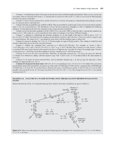
EXAMPLE 6.4 ANALYSIS OF A WATER NETWORK USING THE RELAXATION METHOD OF BALANCING
FLOWS
Balance the network of Fig. 6.13 using the balancing flows method. Necessary calculations are given in Table 6.5.
Elevation of
water table
Take-off F
E = 50´
H 1 H 0
H 0 106´ 50.0´ 69.2´
110´ 1800´−10˝−100 900´−10˝−100 H 1
H 0
H 1
E 0 = 100´
E 0 = 160´ 60.0´ 36.8´
D E E 1 = 119.2´
E 1 = 156´ 2200´−8˝−100
H 1 44.0´ 600´−10˝−120 1000´−10˝−120 50.0´ H 0
H 0 40.0´ H 0 H 1 51.9´ H 1
C 50.0´ 28.9´
Elevation of 1800´−6˝−100 B 30.0´ H 0
Inflow water table E 0 = 150´ 8.9´ H 1 Elevation of
E = 200´
E 1 = 171.1´
A water table
E = 180´
500´−12˝−120
Inflow
′
Figure 6.13 Plan of network analyzed by the method of balancing flows (Example 6.4). Conversion factors: 1 = 1ft = 0.3048 m;
′′
1 = 1in. = 25.4 mm.