Page 267 - Wind Energy Handbook

BLADE LOADS DURING OPERATION 241

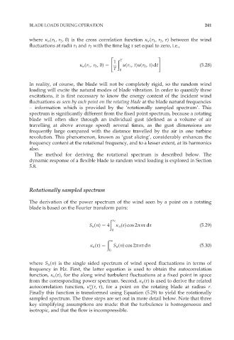
where k u (r 1 , r 2 , 0) is the cross correlation function k u (r 1 , r 2 , ô) between the wind
fluctuations at radii r 1 and r 2 with the time lag ô set equal to zero, i.e.,

" ð #
1 T
k u (r 1 , r 2 ,0) ¼ u(r 1 , t)u(r 2 , t)dt (5:28)
T 0

In reality, of course, the blade will not be completely rigid, so the random wind
loading will excite the natural modes of blade vibration. In order to quantify these
excitations, it is first necessary to know the energy content of the incident wind
fluctuations as seen by each point on the rotating blade at the blade natural frequencies
– information which is provided by the ‘rotationally sampled spectrum’. This
spectrum is significantly different from the fixed point spectrum, because a rotating
blade will often slice through an individual gust (defined as a volume of air
travelling at above average speed) several times, as the gust dimensions are
frequently large compared with the distance travelled by the air in one turbine
revolution. This phenomenon, known as ‘gust slicing’, considerably enhances the
frequency content at the rotational frequency, and to a lesser extent, at its harmonics
also.
The method for deriving the rotational spectrum is described below. The
dynamic response of a flexible blade to random wind loading is explored in Section
5.8.

Rotationally sampled spectrum

The derivation of the power spectrum of the wind seen by a point on a rotating
blade is based on the Fourier transform pairs:

ð 1
S u (n) ¼ 4 k u (ô) cos 2ðnô dô (5:29)
0
ð 1
k u (ô) ¼ S u (n) cos 2ðnô dn (5:30)
0

where S u (n) is the single sided spectrum of wind speed fluctuations in terms of
frequency in Hz. First, the latter equation is used to obtain the autocorrelation
function, k u (ô), for the along wind turbulent fluctuations at a fixed point in space
from the corresponding power spectrum. Second, k u (ô) is used to derive the related
o
autocorrelation function, k (r, ô), for a point on the rotating blade at radius r.
u
Finally this function is transformed using Equation (5.29) to yield the rotationally
sampled spectrum. The three steps are set out in more detail below. Note that three
key simplifying assumptions are made: that the turbulence is homogeneous and
isotropic, and that the flow is incompressible.