Page 270 - Wind Energy Handbook

244 DESIGN LOADS FOR HORIZONTAL-AXIS WIND TURBINES

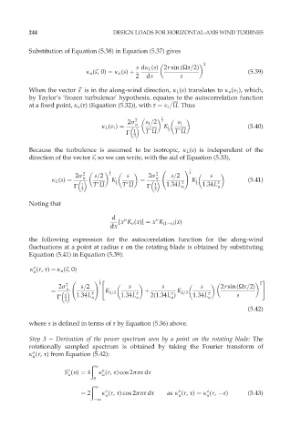
Substitution of Equation (5.38) in Equation (5.37) gives
2
s dk L (s) 2r sin (Ùô=2)
k u (~ s,0) ¼ k L (s) þ (5:39)
s
2 ds s
s
When the vector ~ s is in the along-wind direction, k L (s) translates to k u (s 1 ), which,
by Taylor’s ‘frozen turbulence’ hypothesis, equates to the autocorrelation function
at a fixed point, k u (ô) (Equation (5.32)), with ô ¼ s 1 =U. Thus
1
2ó 2 s 1 =2 3
k L (s 1 ) ¼ K1 s 1 (5:40)
u
ˆ 1 T9U 3 T9U
3
Because the turbulence is assumed to be isotropic, k L (s) is independent of the
direction of the vector ~ s, so we can write, with the aid of Equation (5.33),
s
1 !1
2ó 2 s=2 3 s 2ó 2 s=2 3 s
u
k L (s) ¼ K1 ¼ x K1 x (5:41)
u
ˆ 1 T9U 3 T9U ˆ 1 1:34L u 3 1:34L u
3 3
Noting that
d ı ı
[x K ı (x)] ¼ x K (1 ı) (x)
dx

the following expression for the autocorrelation function for the along-wind
fluctuations at a point at radius r on the rotating blade is obtained by substituting
Equation (5.41) in Equation (5.39):
o
k (r, ô) ¼ k u (~ s,0)
s
u
!1" #
2ó 2 s=2 3 s s s 2rsin(Ùô=2) 2
u
¼ x K 1=3 x þ x K 2=3 x
ˆ 1 1:34L u 1:34L u 2(1:34L ) 1:34L u s
u
3
(5:42)
where s is defined in terms of ô by Equation (5.36) above.

Step 3 – Derivation of the power spectrum seen by a point on the rotating blade: The
rotationally sampled spectrum is obtained by taking the Fourier transform of
o
k (r, ô) from Equation (5.42):
u
ð
1
o
o
S (n) ¼ 4 k (r, ô)cos 2ðnô dô
u
u
0
ð 1
o
o
o
¼ 2 k (r, ô)cos 2ðnô dô as k (r, ô) ¼ k (r, ô) (5:43)
u u u
1