Page 271 - Wind Energy Handbook

BLADE LOADS DURING OPERATION 245

As no analytical solution has been found for the integral, a solution has to be
obtained numerically using a discrete Fourier transform (DFT). First the limits of
o
integration are reduced to T=2, þT=2, as k (r, ô) tends to zero for large ô. Then the
u
o
o
limits of integration are altered to 0, T with k (r, ô) set equal to k (r, T ô) for
u
u
o
ô . T=2, as k (r, ô) is now assumed to be periodic with period T. Thus
u
ð
T
o
o
S (n) ¼ 2 k (r, ô) cos 2 ðnô dô (5:44)
u
u
0
o
where the asterisk denotes that k (r, ô) is ‘reflected’ for T . T=2. The discrete
u
Fourier transform then becomes
2 3
N 1
1 X
o
o
S (n k ) ¼ 2T 4 k (r, pT=N) cos 2ðkp=N 5 (5:45)
u N u
p¼0
o
Here, N is the number of points taken in the time series of k (r, pT=N), and the
u
power spectral density is calculated at the frequencies n k ¼ k=T for k ¼ 0,
1, 2 ... N 1. The expression in square brackets can be evaluated using a standard
fast Fourier transform (FFT), provided N is chosen equal to a power of 2. Clearly N
should be as large as possible if a wide range of frequencies is to be covered at high
o
o
resolution. Just as k (r, ô) is symmetrical about T=2, the values of S (n k ) obtained
u
u
from the FFT are symmetrical about the mid-range frequency of N=(2T), and the
values above this frequency have no real meaning. Moreover, the values of power
spectral density calculated by the DFT at frequencies approaching N=(2T) will be in
error as a result of aliasing, because these are falsely distorted by frequency
o
components above N=(2T) which contribute to the k (r, pT=N) series. Assuming
u
that the calculated spectral densities are valid up to a frequency of N=(4T), then the
selection of T ¼ 100 s and N ¼ 1024 would enable the FFT to give useful results up
to a frequency of about 2.5 Hz at a frequency interval of 0.01 Hz.
Example 5.2
As an illustration, results have been derived for points on a 20 m radius blade
rotating at 30 r.p.m. in a mean wind speed of 8 m=s. Following IEC 61400-1, the
x
integral length scale L is taken as 73.5 m. Figure 5.18 shows how the normalized
u
o
o
2
autocorrelation function, r (r, ô)(¼ k (r, ô)=ó ), for the longitudinal wind fluctua-
u u u
tions varies with the number of rotor revolutions at 20 m, 10 m and 0 m radii. For
r ¼ 10 m, and even more so for r ¼ 20 m, these curves display pronounced peaks
after each full revolution, when the blade may be thought of as encountering the
initial gust or lull once more.
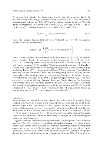
Figure 5.19 shows the corresponding rotationally sampled power spectral density
o
o
2
function, R (r, n)(¼ nS (r, n)=ó ) plotted out against frequency, n, using a loga-
u
u
u
rithmic scale for the latter. It is clear that there is a substantial shift of the frequency
content of the spectrum to the frequency of rotation and, to a lesser degree to its
harmonics, with the extent of the shift increasing with radius. Note that the spectral
density is shown as increasing above a frequency of about 3 Hz. This is an error