Page 338 - Characterization and Properties of Petroleum Fractions - M.R. Riazi

P2: IML/FFX
T1: IML
QC: IML/FFX
P1: IML/FFX
AT029-Manual
AT029-07
AT029-Manual-v7.cls
June 22, 2007
318 CHARACTERIZATION AND PROPERTIES OF PETROLEUM FRACTIONS
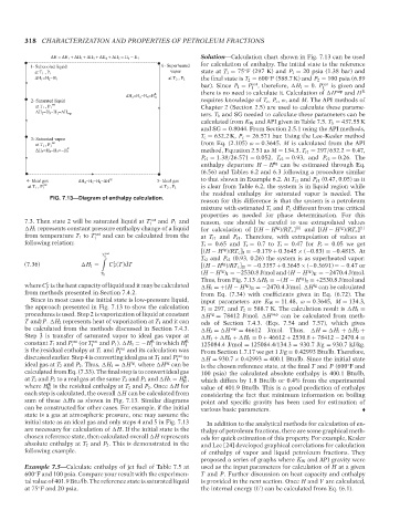
ΔH = ΔH 1 + ΔH 2 + ΔH 3 + ΔH 4 + ΔH 5 = H 6 − H 1 17:40 Solution—Calculation chart shown in Fig. 7.13 can be used
for calculation of enthalpy. The initial state is the reference
1- Subcooled liquid 6- Superheated
vapor state at T 1 = 75 F (297 K) and P 1 = 20 psia (1.38 bar) and
◦
at T 1 , P 1

◦
ΔH 1 =H 2 −H 1 at T 2 , P 2 the final state is T 2 = 600 F (588.7 K) and P 2 = 100 psia (6.89
bar). Since P 1 = P 1 sat , therefore, H 1 = 0. P 1 sat is given and
there is no need to calculate it. Calculation of H vap and H R
R
ΔH 5 =H 6 −H 5 =H II
2- Saturated liquid requires knowledge of T c , P c , ω, and M. The API methods of
sat
at T 1 , P 1 Chapter 2 (Section 2.5) are used to calculate these parame-
ters. T b and SG needed to calculate these parameters can be
ΔH 2 =H 3 −H 2 =ΔH vap
calculated from K W and API given in Table 7.5. T b = 437.55 K
and SG = 0.8044. From Section 2.5.1 using the API methods,
T c = 632.2 K, P c = 26.571 bar. Using the Lee–Kesler method
3- Saturated vapor
sat from Eq. (2.105) ω = 0.3645. M is calculated from the API
at T 1 , P 1
R
ΔH 3 =H 4 −H 3 =−H I method, Equation 2.51 as M = 134.3. T r1 = 297/632.2 = 0.47,
P r1 = 1.38/26.571 = 0.052, T r2 = 0.93, and P r2 = 0.26. The
enthalpy departure H − H ig can be estimated through Eq.
(6.56) and Tables 6.2 and 6.3 following a procedure similar
4- Ideal gas ΔH 4 =H 5 −H 4 =ΔH ig 5- Ideal gas to that shown in Example 6.2. At T r1 and P r1 (0.47, 0.05) as it
sat
at T 1 , P 1 at T 2 , P 2 is clear from Table 6.2, the system is in liquid region while
the residual enthalpy for saturated vapor is needed. The
FIG. 7.13—Diagram of enthalpy calculation.
reason for this difference is that the system is a petroleum
mixture with estimated T c and P c different from true critical
properties as needed for phase determination. For this
7.3. Then state 2 will be saturated liquid at T sat and P 1 and
1 reason, one should be careful to use extrapolated values
H 1 represents constant pressure enthalpy change of a liquid for calculation of [(H − H )/RT c ] (0) and [(H − H )/RT c ] (1)
ig
ig
from temperature T 1 to T sat and can be calculated from the at T r1 and P r1 . Therefore, with extrapolation of values at
1
following relation: T r = 0.65 and T r = 0.7 to T r = 0.47 for P r = 0.05 we get
ig
[(H − H )/RT c ] I =−0.179 + 0.3645 × (−0.83) =−0.4815. At
T sat
T r2 and P r2 (0.93, 0.26) the system is as superheated vapor:
1
L
(7.36) H 1 = C (T)dT [(H − H )/RT c ] II =−0.3357 + 0.3645 × (−0.3691) =− 0.47 or
ig
P
ig
ig
(H − H ) I =−2530.8 J/mol and (H − H ) II =−2470.4 J/mol.
T 1
ig
Thus, from Fig. 7.13 H 3 =−(H − H ) I = +2530.8 J/mol and
L
where C is the heat capacity of liquid and it may be calculated ig ig
P H 5 =+(H − H ) II =−2470.4 J/mol. H can be calculated
from methods presented in Section 7.4.2. from Eq. (7.34) with coefficients given in Eq. (6.72). The
Since in most cases the initial state is low-pressure liquid, input parameters are K W = 11.48, ω = 0.3645, M = 134.3,
the approach presented in Fig. 7.13 to show the calculation T 1 = 297, and T 2 = 588.7 K. The calculation result is H 4 =
procedures is used. Step 2 is vaporization of liquid at constant H = 78412 J/mol. H vap can be calculated from meth-
ig
T and P. H 2 represents heat of vaporization at T 1 and it can ods of Section 7.4.3. (Eqs. 7.54 and 7.57), which gives
be calculated from the methods discussed in Section 7.4.3. H 2 = H vap = 46612 J/mol. Thus, H = H 1 + H 2 +
Step 3 is transfer of saturated vapor to ideal gas vapor at H 3 + H 4 + H 5 = 0 + 46612 + 2530.8 + 78412 − 2470.4 =
R
constant T 1 and P 1 sat (or T 1 sat and P 1 ). H 3 =−H in which H I R 125084.4 J/mol = 125084.4/134.3 = 930.7 J/g = 930.7 kJ/kg.
I
is the residual enthalpy at T 1 and P 1 sat and its calculation was From Section 1.7.17 we get 1 J/g = 0.42993 Btu/lb. Therefore,
discussed earlier. Step 4 is converting ideal gas at T 1 and P 1 sat to H = 930.7 × 0.42993 = 400.1 Btu/lb. Since the initial state
ig
ig
ideal gas at T 2 and P 2 . Thus, H 4 = H , where H can be is the chosen reference state, at the final T and P (600 F and
◦
calculated from Eq. (7.33). The final step is to convert ideal gas 100 psia) the calculated absolute enthalpy is 400.1 Btu/lb,
R
--`,```,`,``````,`,````,```,,-`-`,,`,,`,`,,`---
at T 2 and P 2 to a real gas at the same T 2 and P 2 and H 5 = H , which differs by 1.8 Btu/lb or 0.4% from the experimental
II
R
where H is the residual enthalpy at T 2 and P 2 . Once H for value of 401.9 Btu/lb. This is a good prediction of enthalpy
II
each step is calculated, the overall H can be calculated from considering the fact that minimum information on boiling
sum of these Hs as shown in Fig. 7.13. Similar diagrams point and specific gravity has been used for estimation of
can be constructed for other cases. For example, if the initial various basic parameters.
state is a gas at atmospheric pressure, one may assume the
initial state as an ideal gas and only steps 4 and 5 in Fig. 7.13 In addition to the analytical methods for calculation of en-
are necessary for calculation of H. If the initial state is the thalpy of petroleum fractions, there are some graphical meth-
chosen reference state, then calculated overall H represents ods for quick estimation of this property. For example, Kesler
absolute enthalpy at T 2 and P 2 . This is demonstrated in the and Lee [24] developed graphical correlations for calculation
following example. of enthalpy of vapor and liquid petroleum fractions. They
proposed a series of graphs where K W and API gravity were
Example 7.5—Calculate enthalpy of jet fuel of Table 7.5 at used as the input parameters for calculation of H at a given
600 F and 100 psia. Compare your result with the experimen- T and P. Further discussion on heat capacity and enthalpy
◦
tal value of 401.9 Btu/lb. The reference state is saturated liquid is provided in the next section. Once H and V are calculated,
at 75 F and 20 psia. the internal energy (U) can be calculated from Eq. (6.1).
◦
Copyright ASTM International
Provided by IHS Markit under license with ASTM Licensee=International Dealers Demo/2222333001, User=Anggiansah, Erick
No reproduction or networking permitted without license from IHS Not for Resale, 08/26/2021 21:56:35 MDT