Page 146 - Mechanical Behavior of Materials

Section 4.5 True Stress–Strain Interpretation of Tension Test 147

and Marshal (1952) given at the end of this chapter. The one for steel should not be applied to other
metals except as a rough approximation.

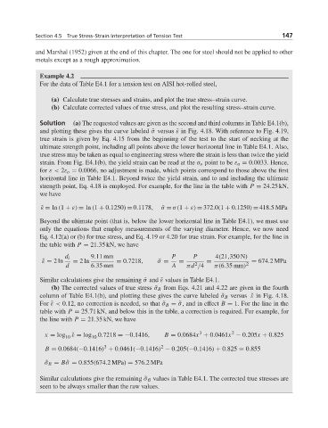
Example 4.2
For the data of Table E4.1 for a tension test on AISI hot-rolled steel,

(a) Calculate true stresses and strains, and plot the true stress–strain curve.
(b) Calculate corrected values of true stress, and plot the resulting stress–strain curve.

Solution (a) The requested values are given as the second and third columns in Table E4.1(b),
and plotting these gives the curve labeled ˜σ versus ˜ε in Fig. 4.18. With reference to Fig. 4.19,
true strain is given by Eq. 4.15 from the beginning of the test to the start of necking at the
ultimate strength point, including all points above the lower horizontal line in Table E4.1. Also,
true stress may be taken as equal to engineering stress where the strain is less than twice the yield
strain. From Fig. E4.1(b), the yield strain can be read at the σ o point to be ε o = 0.0033. Hence,
for ε< 2ε o = 0.0066, no adjustment is made, which points correspond to those above the first
horizontal line in Table E4.1. Beyond twice the yield strain, and to and including the ultimate
strength point, Eq. 4.18 is employed. For example, for the line in the table with P = 24.25 kN,
we have
˜ ε = ln (1 + ε) = ln (1 + 0.1250) = 0.1178, ˜ σ = σ(1 + ε) = 372.0(1 + 0.1250) = 418.5MPa

Beyond the ultimate point (that is, below the lower horizontal line in Table E4.1), we must use
only the equations that employ measurements of the varying diameter. Hence, we now need
Eq. 4.12(a) or (b) for true stress, and Eq. 4.19 or 4.20 for true strain. For example, for the line in
the table with P = 21.35 kN, we have

d i 9.11 mm P P 4(21,350 N)
˜ ε = 2ln = 2ln = 0.7218, ˜ σ = = = = 674.2MPa
2
d 6.35 mm A πd /4 π(6.35 mm) 2
Similar calculations give the remaining ˜σ and ˜ε values in Table E4.1.
(b) The corrected values of true stress ˜σ B from Eqs. 4.21 and 4.22 are given in the fourth
column of Table E4.1(b), and plotting these gives the curve labeled ˜σ B versus ˜ε in Fig. 4.18.
For ˜ε< 0.12, no correction is needed, so that ˜σ B =˜σ, and in effect B = 1. For the line in the
table with P = 25.71 kN, and below this in the table, a correction is required. For example, for
the line with P = 21.35 kN, we have
3
2
x = log ε = log 0.7218 =−0.1416, B = 0.0684x + 0.0461x − 0.205x + 0.825
˜
10
10
2
3
B = 0.0684(−0.1416) + 0.0461(−0.1416) − 0.205(−0.1416) + 0.825 = 0.855
˜ σ B = B ˜σ = 0.855(674.2MPa) = 576.2MPa
Similar calculations give the remaining ˜σ B values in Table E4.1. The corrected true stresses are
seen to be always smaller than the raw values.