Page 149 - Mechanical Behavior of Materials

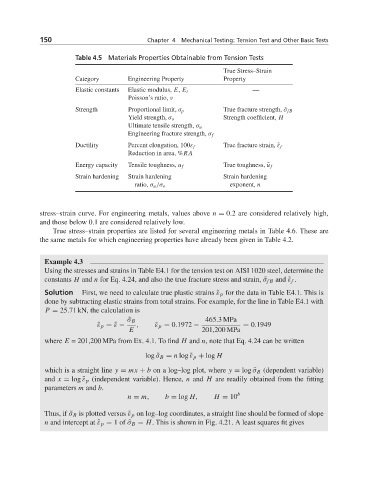
150 Chapter 4 Mechanical Testing: Tension Test and Other Basic Tests

Table 4.5 Materials Properties Obtainable from Tension Tests

True Stress–Strain
Category Engineering Property Property
Elastic constants Elastic modulus, E, E t —
Poisson’s ratio, ν
Strength Proportional limit, σ p True fracture strength, ˜σ fB
Yield strength, σ o Strength coefficient, H
Ultimate tensile strength, σ u
Engineering fracture strength, σ f
Ductility Percent elongation, 100ε f True fracture strain, ˜ε f
Reduction in area, %RA
Energy capacity Tensile toughness, u f True toughness, ˜u f
Strain hardening Strain hardening Strain hardening
ratio, σ u /σ o exponent, n

stress–strain curve. For engineering metals, values above n = 0.2 are considered relatively high,
and those below 0.1 are considered relatively low.
True stress–strain properties are listed for several engineering metals in Table 4.6. These are
the same metals for which engineering properties have already been given in Table 4.2.

Example 4.3
Using the stresses and strains in Table E4.1 for the tension test on AISI 1020 steel, determine the
constants H and n for Eq. 4.24, and also the true fracture stress and strain, ˜σ fB and ˜ε f .
Solution First, we need to calculate true plastic strains ˜ε p for the data in Table E4.1. This is
done by subtracting elastic strains from total strains. For example, for the line in Table E4.1 with
P = 25.71 kN, the calculation is
˜ σ B 465.3MPa
˜ ε p =˜ε − , ˜ ε p = 0.1972 − = 0.1949
E 201,200 MPa
where E = 201,200 MPa from Ex. 4.1. To find H and n, note that Eq. 4.24 can be written
log ˜σ B = n log ˜ε p + log H

which is a straight line y = mx + b on a log–log plot, where y = log ˜σ B (dependent variable)
and x = log ˜ε p (independent variable). Hence, n and H are readily obtained from the fitting
parameters m and b.
n = m, b = log H, H = 10 b

Thus, if ˜σ B is plotted versus ˜ε p on log–log coordinates, a straight line should be formed of slope
n and intercept at ˜ε p = 1of ˜σ B = H. This is shown in Fig. 4.21. A least squares fit gives