Page 147 - Mechanical Behavior of Materials

148 Chapter 4 Mechanical Testing: Tension Test and Other Basic Tests

4.5.5 True Stress–Strain Curves

For true stress–strain curves of metals in the region beyond yielding, the stress versus plastic strain
behavior often fits a power relationship:
˜ σ = H ˜ε n p (4.23)

If stress versus plastic strain is plotted on log–log coordinates, this equation gives a straight line.
The slope is n, which is called the strain hardening exponent. The quantity H, which is called
the strength coefficient, is the intercept at ˜ε p = 1. At large strains during the advanced stages
of necking, Eq. 4.23 should be used with true stresses that have been corrected by means of the
Bridgman factor:
n
˜ σ B = H ˜ε (4.24)
p
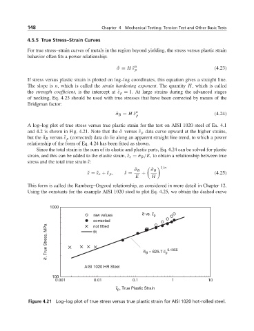
A log–log plot of true stress versus true plastic strain for the test on AISI 1020 steel of Ex. 4.1
and 4.2 is shown in Fig. 4.21. Note that the ˜σ versus ˜ε p data curve upward at the higher strains,
but the ˜σ B versus ˜ε p (corrected) data do lie along an apparent straight line trend, to which a power
relationship of the form of Eq. 4.24 has been fitted as shown.
Since the total strain is the sum of its elastic and plastic parts, Eq. 4.24 can be solved for plastic
strain, and this can be added to the elastic strain, ˜ε e =˜σ B /E, to obtain a relationship between true
stress and the total true strain ˜ε:
1/n

˜ σ B ˜ σ B
˜ ε =˜ε e +˜ε p , ˜ ε = + (4.25)
E H
This form is called the Ramberg–Osgood relationship, as considered in more detail in Chapter 12.
Using the constants for the example AISI 1020 steel to plot Eq. 4.25, we obtain the dashed curve

1000
~ ~
raw values σ vs. ε p
corrected
σ, True Stress, MPa fit ~ ~ 0.1955
not fitted

B
~ σ = 625.7 ε p
AISI 1020 HR Steel
100
0.001 0.01 0.1 1 10
~
ε , True Plastic Strain
p
Figure 4.21 Log–log plot of true stress versus true plastic strain for AISI 1020 hot-rolled steel.