Page 41 - Petroleum Production Engineering, A Computer-Assisted Approach

Guo, Boyun / Computer Assited Petroleum Production Engg 0750682701_chap03 Final Proof page 31 3.1.2007 8:30pm Compositor Name: SJoearun

RESERVOIR DELIVERABILITY 3/31
The real gas pseudo-pressure can be readily determined The flow time required for the pressure funnel to reach the
with the spreadsheet program PseudoPressure.xls. circular boundary can be expressed as
fm o c t r 2
t pss ¼ 1,200 e : (3:7)
3.2.2 Steady-State Flow k
‘‘Steady-state flow’’ is defined as a flow regime where the Because the p e in Eq. (3.6) is not known at any given time,
pressure at any point in the reservoir remains constant the following expression using the average reservoir pres-
over time. This flow condition prevails when the pressure
funnel shown in Fig. 3.1 has propagated to a constant- sure is more useful:
p
pressure boundary. The constant-pressure boundary can q ¼ kh( p p wf ) , (3:8)

be an aquifer or a water injection well. A sketch of the 3
141:2B o m o ln r e þ S
reservoir model is shown in Fig. 3.2, where p e represents r w 4
the pressure at the constant-pressure boundary. Assuming where p ¯ is the average reservoir pressure in psia. Deriv-
single-phase flow, the following theoretical relation can be ations of Eqs. (3.6) and (3.8) are left to readers for exer-
derived from Darcy’s law for an oil reservoir under the cises.
steady-state flow condition due to a circular constant- If the no-flow boundaries delineate a drainage area of
pressure boundary at distance r e from wellbore: noncircular shape, the following equation should be used
for analysis of pseudo–steady-state flow:
kh(p e p wf )
p
q ¼ , (3:5) q ¼ kh( p p wf ) , (3:9)

141:2B o m o ln r e þ S 1 4A
r w ln
141:2B o m o 2 gC A r 2 þ S
w
where ‘‘ln’’ denotes 2.718-based natural logarithm log e . where
Derivation of Eq. (3.5) is left to readers for an exercise.
A ¼ drainage area, ft 2
g ¼ 1:78 ¼ Euler’s constant
3.2.3 Pseudo–Steady-State Flow C A ¼ drainage area shape factor, 31.6 for a circular
‘‘Pseudo–steady-state’’ flow is defined as a flow regime boundary.
where the pressure at any point in the reservoir declines
at the same constant rate over time. This flow condition The value of the shape factor C A can be found from
prevails after the pressure funnel shown in Fig. 3.1 has Fig. 3.4.
propagated to all no-flow boundaries. A no-flow bound- For a gas well located at the center of a circular drainage
ary can be a sealing fault, pinch-out of pay zone, or area, the pseudo–steady-state solution is
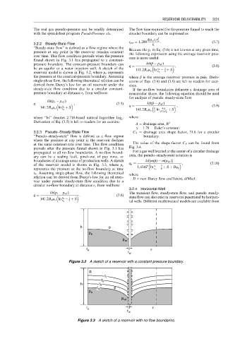
boundaries of drainage areas of production wells. A sketch kh[m( p) m(p wf )]
p
q g ¼ , (3:10)
of the reservoir model is shown in Fig. 3.3, where p e 1,424T ln r e 3
represents the pressure at the no-flow boundary at time r w þ S þ Dq g
4
t 4 . Assuming single-phase flow, the following theoretical where
relation can be derived from Darcy’s law for an oil reser- D ¼ non-Darcy flow coefficient, d/Mscf.
voir under pseudo–steady-state flow condition due to a
circular no-flow boundary at distance r e from wellbore:
3.2.4 Horizontal Well
kh(p e p wf ) The transient flow, steady-state flow, and pseudo–steady-
q ¼ : (3:6) state flow can also exist in reservoirs penetrated by horizon-
1
141:2B o m o ln r e þ S
r w 2 tal wells. Different mathematical models are available from
h p
p e
p wf
r e r
r w

Figure 3.2 A sketch of a reservoir with a constant-pressure boundary.
p i
t 1
t 2
h t 3
t 4 p
p e
p wf
r
r e
r w
Figure 3.3 A sketch of a reservoir with no-flow boundaries.