Page 43 - Petroleum Production Engineering, A Computer-Assisted Approach

Guo, Boyun / Computer Assited Petroleum Production Engg 0750682701_chap03 Final Proof page 33 3.1.2007 8:30pm Compositor Name: SJoearun

RESERVOIR DELIVERABILITY 3/33
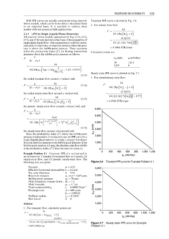
Well IPR curves are usually constructed using reservoir Transient IPR curve is plotted in Fig. 3.6.
inflow models, which can be from either a theoretical basis
or an empirical basis. It is essential to validate these 2. For steady state flow:
models with test points in field applications. kh
J ¼
3.3.1 LPR for Single (Liquid)-Phase Reservoirs 141:2Bm ln r e r w þ S
All reservoir inflow models represented by Eqs. (3.1), (3.3), (8:2)(53)
(3.7), and (3.8) were derived on the basis of the assumption of ¼
single-phase liquid flow. This assumption is valid for under- 141:2(1:1)(1:7) ln 2,980
0:328
saturated oil reservoirs, or reservoir portions where the pres-
¼ 0:1806 STB=d-psi
sure is above the bubble-point pressure. These equations

define the productivity index (J ) for flowing bottom-hole Calculated points are:
pressures above the bubble-point pressure as follows:
q

J ¼ p wf (psi) q o (stb/day)
(p i p wf )
50 1,011
kh
¼ 5,651 0
k
162:6B o m o log t þ log 3:23 þ 0:87S
fm o c t r 2
w Steady state IPR curve is plotted in Fig. 3.7.
(3:15)
3. For pseudosteady state flow:
for radial transient flow around a vertical well,
q kh kh

J ¼ ¼ (3:16) J ¼
3
(p e p wf ) 141:2B o m o ln r e þ S 141:2Bm ln r e þ S
4
r w r w
(8:2)(53)
for radial steady-state flow around a vertical well, ¼
141:2(1:1)(1:7) ln 2,980 0:75
q kh 0:328

J ¼ ¼ (3:17)
p
( p p wf ) 1 4A ¼ 0:1968 STB=d-psi
141:2B o m o 2 ln gC A r 2 þ S
w
for pseudo–steady-state flow around a vertical well, and
q 6,000

J ¼
(p e p wf )
5,000
k H h
¼ p ffiffiffiffiffiffiffiffiffiffiffiffiffiffiffiffi h i
aþ a 2 (L=2) 2 I ani h I ani h
141:2Bm ln þ ln 4,000
L=2 L r w (I ani þ1)
(3:18) p wf (psia) 3,000
for steady-state flow around a horizontal well.

Since the productivity index (J ) above the bubble-point
pressure isindependent of productionrate, the IPR curve for a 2,000
single (liquid)-phase reservoir is simply a straight line drawn
from the reservoir pressure to the bubble-point pressure. If the 1,000
bubble-point pressure is 0 psig, the absolute open flow (AOF)

is the productivity index (J ) times the reservoir pressure. 0
0 200 400 600 800 1,000 1,200
Example Problem 3.1 Construct IPR of a vertical well in
an oil reservoir. Consider (1) transient flow at 1 month, (2) q o (stb/day)
steady-state flow, and (3) pseudo–steady-state flow. The
following data are given: Figure 3.6 Transient IPR curve for Example Problem 3.1.
Porosity: f ¼ 0:19 6,000
Effective horizontal permeability:k ¼ 8:2md
Pay zone thickness: h ¼ 53 ft
Reservoir pressure: p e or p ¼ 5,651 psia 5,000
p
Bubble-point pressure: p b ¼ 50 psia
Fluid formation volume factor:, B o ¼ 1:1 4,000
Fluid viscosity: m o ¼ 1:7cp
Total compressibility, c t ¼ 0:0000129 psi 1
Drainage area: A ¼ 640 acres p wf (psia) 3,000
(r e ¼ 2,980 ft)
Wellbore radius: r w ¼ 0:328 ft 2,000
Skin factor: S ¼ 0
Solution 1,000
1. For transient flow, calculated points are
0
kh

J ¼ 0 200 400 600 800 1,000 1,200
162:6Bm log t þ log fmc t r 2 3:23 q o (stb/day)
w
(8:2)(53)
¼
(8:2)
162:6(1:1)(1:7) log [( (30)(24)] þ log (0:19)(1:7)(0:0000129)(0:328) 2 3:23 Figure 3.7 Steady-state IPR curve for Example
¼ 0:2075 STB=d-psi Problem 3.1.