Page 46 - Petroleum Production Engineering, A Computer-Assisted Approach

Guo, Boyun / Computer Assited Petroleum Production Engg 0750682701_chap03 Final Proof page 36 3.1.2007 8:30pm Compositor Name: SJoearun

3/36 PETROLEUM PRODUCTION ENGINEERING FUNDAMENTALS

Forapartialtwo-phasereservoir,modelconstantJ inthe Well B:
generalizedVogelequationmustbedeterminedbasedonthe

range of tested flowing bottom-hole pressure. If the tested J ¼ q 1 2
flowing bottom-hole pressure is greater than bubble-point ( p p b ) þ p b 1 0:2 p wf 1 0:8 p wf 1
p

pressure, the model constant J should be determined by 1:8 p b p b

J ¼ q 1 : (3:30) ¼ 900
p
( p p wf 1 ) 2
(5,000 3,000) þ 3,000 1 0:2 2,000 0:8 2,000
3,000
3,000
1:8
If the tested flowing bottom-hole pressure is less than

bubble-point pressure, the model constant J should be ¼ 0:3156 stb=day-psi
determined using Eq. (3.28), that is,
Calculated points are
!

J ¼ " q 1 2 # :
p b p wf 1 p wf 1
p
( p p b ) þ 1 0:2 0:8 p wf (psia) q (stb/day)
1:8 p b p b
0 1,157
(3:31) 500 1,128
Example Problem 3.4 Construct IPR of two wells in an 1,000 1,075
undersaturated oil reservoir using the generalized Vogel 1,500 999
equation. The following data are given: 2,000 900
2,500 777
Reservoir pressure: p p ¼ 5,000 psia 3,000 631
Bubble point pressure: p b ¼ 3,000 psia 5,000 0
Tested flowing bottom-hole
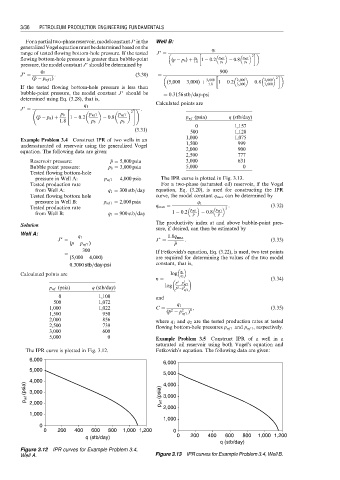
pressure in Well A: p wf 1 ¼ 4,000 psia The IPR curve is plotted in Fig. 3.13.
Tested production rate For a two-phase (saturated oil) reservoir, if the Vogel
from Well A: q 1 ¼ 300 stb=day equation, Eq. (3.20), is used for constructing the IPR
Tested flowing bottom hole curve, the model constant q max can be determined by
pressure in Well B: p wf 1 ¼ 2,000 psia q 1
Tested production rate q max ¼ p wf 1 p wf 1 2 : (3:32)
from Well B: q 1 ¼ 900 stb=day 1 0:2 p p 0:8 p p
The productivity index at and above bubble-point pres-
Solution
sure, if desired, can then be estimated by
Well A:

J ¼ q 1 J ¼ 1:8q max : (3:33)
( p p wf 1 ) p p
p
300 If Fetkovich’s equation, Eq. (3.22), is used, two test points
¼
(5,000 4,000) are required for determining the values of the two model
¼ 0:3000 stb=day-psi constant, that is,

Calculated points are log q 1 q 2
n ¼ (3:34)
p p 2 p 2
log wf 1
p wf (psia) q (stb/day) p p 2 p 2
wf 2
0 1,100 and
500 1,072
1,000 1,022 C ¼ 2 q 1 2 n , (3:35)
p
1,500 950 ( p p wf 1 )
2,000 856 where q 1 and q 2 are the tested production rates at tested
2,500 739 flowing bottom-hole pressures p wf 1 and p wf 1 , respectively.
3,000 600
5,000 0 Example Problem 3.5 Construct IPR of a well in a
saturated oil reservoir using both Vogel’s equation and
The IPR curve is plotted in Fig. 3.12. Fetkovich’s equation. The following data are given:
6,000
6,000
5,000
5,000
4,000 4,000
p wf (psia) 3,000 p wf (psia) 3,000
2,000
2,000
1,000
1,000
0
0 200 400 600 800 1,000 1,200 0
q (stb/day) 0 200 400 600 800 1,000 1,200
q (stb/day)
Figure 3.12 IPR curves for Example Problem 3.4,
Well A. Figure 3.13 IPR curves for Example Problem 3.4, Well B.