Page 44 - Petroleum Production Engineering, A Computer-Assisted Approach

Guo, Boyun / Computer Assited Petroleum Production Engg 0750682701_chap03 Final Proof page 34 3.1.2007 8:30pm Compositor Name: SJoearun

3/34 PETROLEUM PRODUCTION ENGINEERING FUNDAMENTALS
6,000 or
2
2
n
p
q ¼ C( p p ) , (3:23)
5,000 wf
4,000 where C and n are empirical constants and is related to
p wf (psia) 3,000 3.5, the Fetkovich equation with two constants is more
2n
q max by C ¼ q max = p . As illustrated in Example Problem
p
accurate than Vogel’s equation IPR modeling.
2,000 Again, Eqs. (3.19) and (3.23) are valid for average reservoir
pressure p being at and below the initial bubble-point pres-
p
sure. Equation (3.23) is often used for gas reservoirs.
1,000
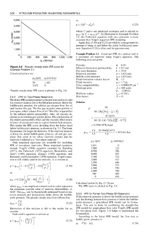
Example Problem 3.2 Construct IPR of a vertical well in
0
0 200 400 600 800 1,000 1,200 a saturated oil reservoir using Vogel’s equation. The
q o (stb/day) following data are given:
Porosity: f ¼ 0:19
Figure 3.8 Pseudo–steady-state IPR curve for Effective horizontal permeability: k ¼ 8.2 md
Example Problem 3.1.
Pay zone thickness: h ¼ 53 ft
Calculated points are: Reservoir pressure: p p ¼ 5,651 psia
Bubble point pressure: p b¼ 5,651 psia
p wf (psi) q o (stb/day)
Fluid formation volume factor: B o¼ 1:1
50 1,102 Fluid viscosity: m o ¼ 1:7cp
5,651 0 Total compressibility: c t ¼ 0:0000129 psi 1
Drainage area: A ¼ 640 acres
Pseudo–steady-state IPR curve is plotted in Fig. 3.8. (r e ¼ 2,980 ft)
Wellbore radius: r w ¼ 0:328 ft
3.3.2 LPR for Two-Phase Reservoirs Skin factor: S ¼ 0
The linear IPR model presented in the previous section is valid
for pressure values as low as bubble-point pressure. Below the Solution
bubble-point pressure, the solution gas escapes from the oil
and become free gas. The free gas occupies some portion of J ¼ kh

3
pore space, which reduces flow of oil. This effect is quantified 141:2Bm ln r e þ S
4
by the reduced relative permeability. Also, oil viscosity in- r w
creases as its solution gas content drops. The combination of ¼ (8:2)(53)

the relative permeability effect and the viscosity effect results 141:2(1:1)(1:7) ln 2,980 0:75
in lower oil production rate at a given bottom-hole pressure. 0:328
This makes the IPR curve deviating from the linear trend ¼ 0:1968 STB=d-psi
below bubble-point pressure, as shown in Fig. 3.5. The lower
the pressure, the larger the deviation. If the reservoir pressure q max ¼ J p p ¼ (0:1968)(5,651) ¼ 618 stb=day
is below the initial bubble-point pressure, oil and gas two- 1:8 1:8
phase flow exists in the whole reservoir domain and the
reservoir is referred as a ‘‘two-phase reservoir.’’ p wf (psi) q o (stb/day)
Only empirical equations are available for modeling
IPR of two-phase reservoirs. These empirical equations 5,651 0
include Vogel’s (1968) equation extended by Standing 5,000 122
(1971), the Fetkovich (1973) equation, Bandakhlia and 4,500 206
Aziz’s (1989) equation, Zhang’s (1992) equation, and 4,000 283
Retnanto and Economides’ (1998) equation. Vogel’s equa- 3,500 352
tion is still widely used in the industry. It is written as 3,000 413
" 2 # 2,500 466
p wf p wf 2,000 512
q ¼ q max 1 0:2 0:8 (3:19)
p p p p 1,500 550
1,000 580
or 500 603
" s ffiffiffiffiffiffiffiffiffiffiffiffiffiffiffiffiffiffiffiffiffiffiffiffiffiffiffiffiffiffiffiffi # 0 618

q
p wf ¼ 0:125 p p 81 80 1 , (3:20)
q max
Calculated points by Eq. (3.19) are
where q max is an empirical constant and its value represents The IPR curve is plotted in Fig. 3.9.
the maximum possible value of reservoir deliverability, or
AOF. The q max can be theoretically estimated based on res-
ervoir pressure and productivity index above the bubble- 3.3.3 IPR for Partial Two-Phase Oil Reservoirs
point pressure. The pseudo–steady-state flow follows that If the reservoir pressure is above the bubble-point pressure
and the flowing bottom-hole pressure is below the bubble-

J p p
q max ¼ : (3:21) point pressure, a generalized IPR model can be formu-
1:8 lated. This can be done by combining the straight-line
Derivation of this relation is left to the reader for an IPR model for single-phase flow with Vogel’s IPR model
exercise. for two-phase flow. Figure 3.10 helps to understand the
Fetkovich’s equation is written as formulation.
" 2 # n According to the linear IPR model, the flow rate at
p wf bubble-point pressure is
q ¼ q max 1 (3:22)
p p q b ¼ J ( p p b ), (3:24)

p