Page 45 - Petroleum Production Engineering, A Computer-Assisted Approach

Guo, Boyun / Computer Assited Petroleum Production Engg 0750682701_chap03 Final Proof page 35 3.1.2007 8:30pm Compositor Name: SJoearun

RESERVOIR DELIVERABILITY 3/35
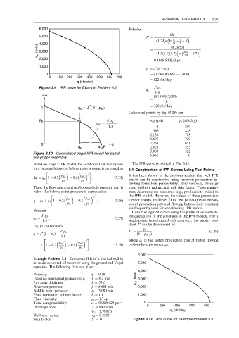
6,000 Solution
kh
5,000 J ¼

3
141:2Bm ln r e þ S
4
r w
4,000 (8:2)(53)
p wf (psia) 3,000 ¼ 141:2(1:1)(1:7) ln 2,980 0:75

0:328
2,000
¼ 0:1968 STB=d-psi
1,000
q b ¼ J ( p p b )
p
0 ¼ (0:1968)(5,651 3,000)
0 100 200 300 400 500 600 700
¼ 522 sbt=day
q (stb/day)

Figure 3.9 IPR curve for Example Problem 3.2. J p b
q v ¼
1:8
p wf (0:1968)(3,000)
¼
1:8
*
p i q b = J ( p − p b ) ¼ 328 stb=day
Calculated points by Eq. (3.28) are
*
p b J p p wf (psi) q o (stb/day)
q V = b
1.8 0 850
565 828
1,130 788
1,695 729
0 q 2,260 651
q b AOF 2,826 555
3,000 522
Figure 3.10 Generalized Vogel IPR model for partial 5,651 0
two-phase reservoirs.
Based on Vogel’s IPR model, the additional flow rate caused The IPR curve is plotted in Fig. 3.11.
by a pressure below the bubble-point pressure is expressed as
" 2 # 3.4 Construction of IPR Curves Using Test Points
p wf p wf It has been shown in the previous section that well IPR
Dq ¼ q v 1 0:2 0:8 : (3:25)
p b p b curves can be constructed using reservoir parameters in-
cluding formation permeability, fluid viscosity, drainage
Thus, the flow rate at a given bottom-hole pressure that is area, wellbore radius, and well skin factor. These param-
below the bubble-point pressure is expressed as eters determine the constants (e.g., productivity index) in
" 2 # the IPR model. However, the values of these parameters
p wf p wf are not always available. Thus, test points (measured val-
q ¼ q b þ q v 1 0:2 0:8 : (3:26)
p b p b ues of production rate and flowing bottom-hole pressure)
are frequently used for constructing IPR curves.
Because
Constructing IPR curves using test points involves back-

J p b ing-calculation of the constants in the IPR models. For a
q v ¼ , (3:27)
1:8 single-phase (unsaturated oil) reservoir, the model con-

stant J can be determined by
Eq. (3.26) becomes

J ¼ q 1 , (3:29)

p
q ¼ J ( p p b ) þ J p b ( p p wf 1 )
p
1:8
" 2 # where q 1 is the tested production rate at tested flowing
p wf p wf
1 0:2 0:8 : (3:28) bottom-hole pressure p wf 1 .
p b p b
6,000
Example Problem 3.3 Construct IPR of a vertical well in
an undersaturated oil reservoir using the generalized Vogel 5,000
equation. The following data are given:
4,000
Porosity: f ¼ 0:19
Effective horizontal permeability: k ¼ 8.2 md p wf (psia) 3,000
Pay zone thickness: h ¼ 53 ft
Reservoir pressure: p p ¼ 5,651 psia 2,000
Bubble point pressure: p b¼ 3,000 psia
Fluid formation volume factor: B o¼ 1:1 1,000
Fluid viscosity: m o ¼ 1:7cp
Total compressibility: c t ¼ 0:0000129 psi 1 0
Drainage area: A ¼ 640 acres 0 200 400 600 800
(r e ¼ 2,980 ft) q o (stb/day)
Wellbore radius: r w ¼ 0:328 ft
Skin factor: S ¼ 0 Figure 3.11 IPR curve for Example Problem 3.3.