Page 52 - Petroleum Production Engineering, A Computer-Assisted Approach

Guo, Boyun / Computer Assited Petroleum Production Engg 0750682701_chap03 Final Proof page 42 3.1.2007 8:30pm Compositor Name: SJoearun

3/42 PETROLEUM PRODUCTION ENGINEERING FUNDAMENTALS
0
Solution The value of J at 1,500 psia is References
o
bandakhlia, h. and aziz, k. Inflow performance relation-
0 4 1,500
J ¼ 5 10 ship for solution-gas drive horizontal wells. Presented
o 2,000
at the 64th SPE Annual Technical Conference and
2
¼ 3:75 10 4 stb=day (psia) , Exhibition held 8–11 October 1989, in San Antonio,
0
and the value of J at 1,000 psia is Texas. Paper SPE 19823.
o
chang, m. Analysis of inflow performance simulation of
0 4 1,000 4 2
J ¼ 5 10 ¼ 2:5 10 stb=day(psia) : solution-gas drive for horizontal/slant vertical wells.
o
2,000
Presented at the SPE Rocky Mountain Regional Meet-
0
Using the above values for J and the accompanying p e in ing held 18–21 May 1992, in Casper, Wyoming. Paper
o
Eq. (3.46), the following data points are calculated: SPE 24352.
dietz, d.n. Determination of average reservoir pressure
p e ¼ 2,000 psig p e ¼ 1,500 psig p e ¼ 1,000 psig from build-up surveys. J. Pet. Tech. 1965; August.
dake, l.p. Fundamentals of Reservoir Engineering. New
q q q
p wf p wf p wf York: Elsevier, 1978.
ðpsigÞ (stb/day) ðpsigÞ (stb/day) ðpsigÞ (stb/day)
earlougher, r.c. Advances in Well Test Analysis. Dallad:
2,000 0 1,500 0 1,000 0 Society of Petroleum Engineers, 1977.
1,800 380 1,350 160 900 48 el-banbi, a.h. and wattenbarger, r.a. Analysis of com-
1,600 720 1,200 304 800 90 mingled tight gas reservoirs. Presented at the SPE
1,400 1,020 1,050 430 700 128 Annual Technical Conference and Exhibition held 6–
1,200 1,280 900 540 600 160 9 October 1996, in Denver, Colorado. Paper SPE
1,000 1,500 750 633 500 188 36736.
800 1,680 600 709 400 210
el-banbi, a.h. and wattenbarger, r.a. Analysis of com-
600 1,820 450 768 300 228
400 1,920 300 810 200 240 mingled gas reservoirs with variable bottom-hole flow-
200 1,980 150 835 100 248 ing pressure and non-Darcy flow. Presented at the SPE
0 2,000 0 844 0 250 Annual Technical Conference and Exhibition held 5–8
October 1997, in San Antonio, Texas. Paper SPE
38866.
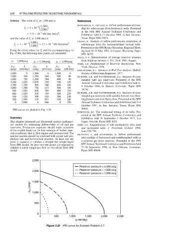
IPR curves are plotted in Fig. 3.20.
fetkovich, m.j. The isochronal testing of oil wells. Pre-
sented at the SPE Annual Technical Conference and
Summary Exhibition held 30 September–3 October 1973, Las
This chapter presented and illustrated various mathemat- Vegas, Nevada. Paper SPE 4529.
ical models for estimating deliverability of oil and gas joshi, s.d. Augmentation of well productivity with slant
reservoirs. Production engineers should make selections and horizontal wells. J. Petroleum Technol. 1988;
of the models based on the best estimate of his/her reser- June:729–739.
voir conditions, that is, flow regime and pressure level. The retnanto, a. and economides, m. Inflow performance
selected models should be validated with actual well pro-
duction rate and bottom-hole pressure. At least one test relationships of horizontal and multibranched wells in
point is required to validate a straight-line (single-liquid a solution gas drive reservoir. Presented at the 1998
flow) IPR model. At least two test points are required to SPE Annual Technical Conference and Exhibition held
validate a curvic (single-gas flow or two-phase flow) IPR 27–30 September 1998, in New Orleans, Louisiana.
model. Paper SPE 49054.
2,500
Reservoir pressure = 2,000 psig
Reservoir pressure = 1,500 psig
2,000
Reservoir pressure = 1,000 psig
p wf (psig) 1,500

1,000

500

0
0 500 1,000 1,500 2,000 2,500
q (stb/day)
Figure 3.20 IPR curves for Example Problem 3.7.