Page 334 - Acquisition and Processing of Marine Seismic Data

6.3 SPIKING DECONVOLUTION 325

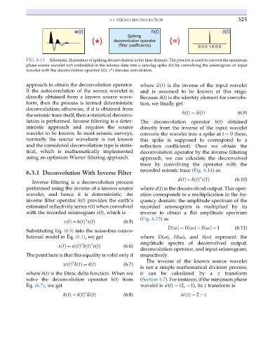
FIG. 6.13 Schematic illustration of spiking deconvolution in the time domain. The process is used to convert the minimum
phase source wavelet w(t) embedded in the seismic data into a zero-lag spike δ(t) by convolving the seismogram or input
wavelet with the deconvolution operator h(t). (*) denotes convolution.

approach to obtain the deconvolution operator. where e wtðÞ is the inverse of the input wavelet
If the autocorrelation of the source wavelet is and is assumed to be known at this stage.
directly obtained from a known source wave- Because δ(t) is the identity element for convolu-
form, then the process is termed deterministic tion, we finally get
deconvolution; otherwise, if it is obtained from
the seismic trace itself, then a statistical deconvo- htðÞ ¼ e wtðÞ (6.9)
lution is performed. Inverse filtering is a deter- The deconvolution operator h(t) obtained
ministic approach and requires the source directly from the inverse of the input wavelet
wavelet to be known. In most seismic surveys, converts the wavelet into a spike at t ¼ 0 (here,
normally the source waveform is not known this spike is supposed to correspond to a
and the considered deconvolution type is statis- reflection coefficient). Once we obtain the
tical, which is mathematically implemented deconvolution operator by the inverse filtering
using an optimum Wiener filtering approach. approach, we can calculate the deconvolved
trace by convolving the operator with the
recorded seismic trace (Fig. 6.14)as
6.3.1 Deconvolution With Inverse Filter
∗ (6.10)
Inverse filtering is a deconvolution process dtðÞ ¼ htðÞ stðÞ
performed using the inverse of a known source where d(t) is the deconvolved output. This oper-
wavelet, and hence it is deterministic. An ation corresponds to a multiplication in the fre-
inverse filter operator h(t) provides the earth’s quency domain: the amplitude spectrum of the
estimated reflectivity series r(t) when convolved recorded seismogram is multiplied by its
with the recorded seismogram s(t), which is inverse to obtain a flat amplitude spectrum
∗ (Fig. 6.15)as
rtðÞ ¼ htðÞ stðÞ (6.5)
D ωðÞ ¼ H ωðÞ S ωðÞ ¼ 1 (6.11)
Substituting Eq. (6.5) into the noise-free convo-
lutional model in Eq. (6.1), we get where D(ω), H(ω), and S(ω) represent the
∗ ∗ amplitude spectra of deconvolved output,
stðÞ ¼ wtðÞ htðÞ stðÞ (6.6)
deconvolution operator, and input seismogram,
The point here is that this equality is valid only if respectively.
The inverse of the known source wavelet
∗
wtðÞ htðÞ ¼ δ tðÞ (6.7)
is not a simple mathematical division process;
where δ(t) is the Dirac delta function. When we it can be calculated by a z transform
solve the deconvolution operator h(t) from (Section 4.7). For instance, if the minimum phase
Eq. (6.7), we get wavelet is w(t) ¼ (2, 1), its z transform is
∗
htðÞ ¼ δ tðÞ e wtðÞ (6.8) wzðÞ ¼ 2 z