Page 335 - Acquisition and Processing of Marine Seismic Data

326 6. DECONVOLUTION

FIG. 6.14 Block diagram of spiking deconvolution
application in the time domain by inverse filtering. (*)
denotes convolution.

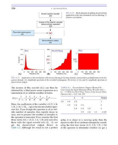
FIG. 6.15 Application of deconvolution with inverse filtering in the time domain corresponds to multiplication in the fre-
quency domain. (A) Amplitude spectrum of the recorded seismogram, (B) inverse of (A), and (C) amplitude spectrum of
deconvolved output.

The inverse of this wavelet e wzðÞ can then be TABLE 6.2 Deconvolution Output Obtained by
obtained by a MacLaurin series expansion as a Convolving the Input Minimum Phase Wavelet w(t) ¼
(2, 1) With the First Three Terms of the Inverse Filter
summation of an infinite number of terms
Operator h(t) ¼ (1/2, 1/4, 1/8)
1 1 1 1 2 1 3 1 4
e wzðÞ ¼ ¼ + z + z + z + z + ⋯⋯: 2 21 Output
2 z 2 4 8 16 32
1/8 1/4 1/2 1
Here, the coefficients of the variable z (1/2, 1/4, 1/8 1/4 1/2 0
1/8, 1/16, 1/32,…) give the deconvolution oper-
ator h(t). Even though the operator is of an infi- 1/8 1/4 1/2 0
nite number of samples, they rapidly decay to 1/8 1/4 1/2 0.125
zero, and in practice the number of samples in
the operator is truncated. If we consider the first
three terms h(t) ¼ (1/2, 1/4, 1/8) and convolve spike, it is closer to a zero-lag spike than the
them with the input wavelet w(t)¼(2, 1), we input wavelet. If we continue attempts by consid-
get the deconvolved output shown in ering the first four terms (1/2, 1/4, 1/8, 1/16)
Table 6.2. Although the result is not a perfect of the operator to determine whether we get a