Page 340 - Acquisition and Processing of Marine Seismic Data

6.3 SPIKING DECONVOLUTION 331

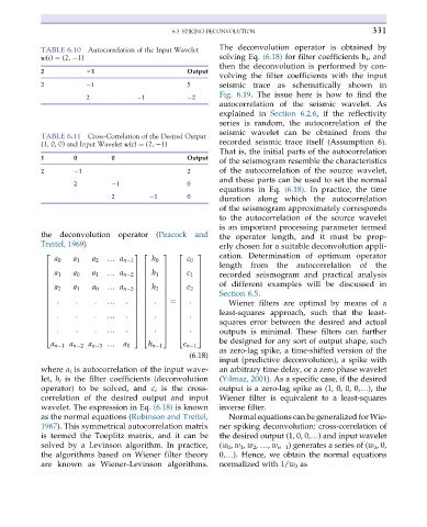
TABLE 6.10 Autocorrelation of the Input Wavelet The deconvolution operator is obtained by
w(t) ¼ (2, 1) solving Eq. (6.18) for filter coefficients h i ,and
then the deconvolution is performed by con-
volving the filter coefficients with the input
2 21 Output
2 1 5 seismic trace as schematically shown in
Fig. 6.19. The issue here is how to find the
2 1 2
autocorrelation of the seismic wavelet. As
explained in Section 6.2.6,ifthereflectivity
series is random, the autocorrelation of the
seismic wavelet can be obtained from the
TABLE 6.11 Cross-Correlation of the Desired Output
(1, 0, 0) and Input Wavelet w(t) ¼ (2, 1) recorded seismic trace itself (Assumption 6).
That is, the initial parts of the autocorrelation
of the seismogram resemble the characteristics
1 0 0 Output
2 1 2 of the autocorrelation of the source wavelet,
and these parts can be used to set the normal
2 1 0
equations in Eq. (6.18).Inpractice, thetime
2 1 0
duration along which the autocorrelation
of the seismogram approximately corresponds
to the autocorrelation of the source wavelet
is an important processing parameter termed
the deconvolution operator (Peacock and the operator length, and it must be prop-
Treitel, 1969) erly chosen for a suitable deconvolution appli-
cation. Determination of optimum operator
2 3 2 3 2 3
a 0 a 1 a 2 … a n 1 h 0 c 0
length from the autocorrelation of the
6 7 6 7 6 7
a 1 a 0 a 1 … a n 2 h 1 c 1 recorded seismogram and practical analysis
6 7 6 7 6 7
6 7 6 7 6 7
of different examples will be discussed in
6 7 6 7 6 7
a 2 a 1 a 0 … a n 3 h 2 c 2
6 7 6 7 6 7
Section 6.5.
6 7 6 7 6 7
6 7 6 7 6 7
: : : : : :
6 … 7 6 7 ¼ 6 7 Wiener filters are optimal by means of a
6 7 6 7 6 7
6 7 6 7 6 7 least-squares approach, such that the least-
: : : : : :
6 … 7 6 7 6 7
squares error between the desired and actual
6 7 6 7 6 7
6 7 6 7 6 7
: : : : : :
6 … 7 6 7 6 7 outputs is minimal. These filters can further
4 5 4 5 4 5
be designed for any sort of output shape, such
a 0 h n 1 c n 1
a n 1 a n 2 a n 3 …
as zero-lag spike, a time-shifted version of the
(6.18)
input (predictive deconvolution), a spike with
where a i is autocorrelation of the input wave- an arbitrary time delay, or a zero phase wavelet
let, h i is the filter coefficients (deconvolution (Yılmaz, 2001). As a specific case, if the desired
operator) to be solved, and c i is the cross- output is a zero-lag spike as (1, 0, 0, 0,…), the
correlation of the desired output and input Wiener filter is equivalent to a least-squares
wavelet. The expression in Eq. (6.18) is known inverse filter.
as the normal equations (Robinson and Treitel, Normal equations can be generalized for Wie-
1967). This symmetrical autocorrelation matrix ner spiking deconvolution: cross-correlation of
is termed the Toeplitz matrix, and it can be the desired output (1, 0, 0,…) and input wavelet
solved by a Levinson algorithm. In practice, (w 0 , w 1 , w 2 , …, w n 1 ) generates a series of (w 0 ,0,
the algorithms based on Wiener filter theory 0,…). Hence, we obtain the normal equations
are known as Wiener-Levinson algorithms. normalized with 1/w 0 as