Page 344 - Acquisition and Processing of Marine Seismic Data

6.4 PREDICTIVE DECONVOLUTION 335

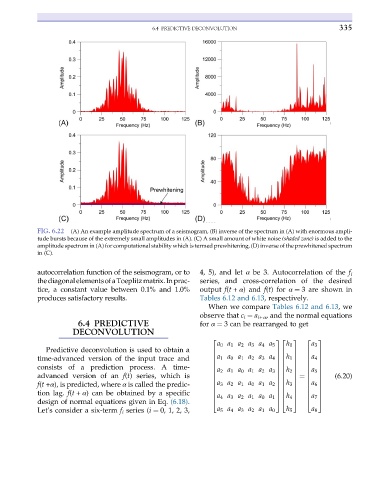
FIG. 6.22 (A) An example amplitude spectrum of a seismogram, (B) inverse of the spectrum in (A) with enormous ampli-
tude bursts because of the extremely small amplitudes in (A). (C) A small amount of white noise (shaded zone) is added to the
amplitude spectrum in (A) for computational stability which is termed prewhitening, (D) inverse of the prewhitened spectrum
in (C).

autocorrelation function of the seismogram, or to 4, 5), and let α be 3. Autocorrelation of the f i
thediagonalelementsofaToeplitzmatrix.Inprac- series, and cross-correlation of the desired
tice, a constant value between 0.1% and 1.0% output f(t + α) and f(t) for α ¼ 3 are shown in
produces satisfactory results. Tables 6.12 and 6.13, respectively.
When we compare Tables 6.12 and 6.13,we
observe that c i ¼ a i+α , and the normal equations
6.4 PREDICTIVE for α ¼ 3 can be rearranged to get
DECONVOLUTION
2 32 3 2 3
a 0 a 1 a 2 a 3 a 4 a 5 h 0 a 3
Predictive deconvolution is used to obtain a
6 76 7 6 7
time-advanced version of the input trace and 6 a 1 a 0 a 1 a 2 a 3 a 4 7 h 1 7 6 a 4 7
6
6 76 7 6 7
consists of a prediction process. A time- 6 76 7 6 7
6 a 2 a 1 a 0 a 1 a 2 a 3 76 h 2 7 6 a 5 7
advanced version of an f(t) series, which is 6 76 7 6 7 (6.20)
6 76 7 ¼ 6 7
f(t +α), is predicted, where α is called the predic- 6 a 3 a 2 a 1 a 0 a 1 a 2 76 h 3 7 6 a 6 7
76
7
7
6
6
tion lag. f(t + α) can be obtained by a specific 6 76 7 6 7
7
6
76
6
7
design of normal equations given in Eq. (6.18). 4 a 4 a 3 a 2 a 1 a 0 a 1 54 h 4 5 4 a 7 5
Let’s consider a six-term f i series (i ¼ 0, 1, 2, 3, a 5 a 4 a 3 a 2 a 1 a 0 h 5 a 8