
Page 337 - Acquisition and Processing of Marine Seismic Data
P. 337
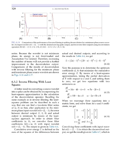
328 6. DECONVOLUTION
FIG. 6.16 Comparison of the performance of inverse filtering in spiking deconvolution for a minimum phase source wave-
let. (A) Input wavelet w(t) ¼ (2, 1) with the desired zero lag spike output, and its inverse filter outputs using deconvolution
operators (B) h(t) ¼ (1/2, 1/4, 1/8), (C) h(t) ¼ (1/2, 1/4, 1/8, 1/16).
series. Because the wavelet is not minimum actual and desired outputs, and according to
phase, its energy is not front-loaded and the results in Table 6.6, we get
Assumption 5 is violated. Therefore, increasing
2 2 2
½
½
ð
the number of terms will not provide a further E ¼ 2aðÞ 1 +2b að½ Þ 0 + bÞ 0
improvement in the deconvolution output. (6.12)
Comparisons of the results of deconvolution
Now the purpose is to determine the optimum
with inverse filtering for the minimum phase coefficients (a, b) that minimize the cumulative
and maximum phase source wavelets are shown error energy E. By means of a least-squares
in Figs. 6.16 and 6.17.
approximation, taking the partial derivatives
of E with respect to a and b, and setting them
6.3.2 Inverse Filtering With Least to zero, we get two equations with two
Squares unknowns as
∂E
A better result in converting a source wavelet ¼ 10a 4b 4 ¼ 0 ) 5a 2b ¼ 2
into a spike can be obtained by incorporating the ∂a (6.13)
least-squares approximation in the calculation ∂E
¼ 10b 4a ¼ 0 ) 2a +5b ¼ 0
of the deconvolution operator. Recalling the ∂b
same example as in inverse filtering, the least-
When we rearrange these equations into a
squares problem can be described in such a
matrix form, and solve them for a and b coeffi-
way that one can find a two-term filter series
cients, we get
of (a, b) so that, after application to the mini-
2 3 2 3 2 3
mum phase input wavelet w(t)¼(2, 1), the error 5 2 a 2
between desired output (1, 0, 0) and actual 6 7 6 7 6 7
4 5 4 5 ¼ 4 5
output is minimum by means of the least- 2 5 b 0 (6.14)
squares approach. In order to obtain filter 10 4
coefficients (a, b), we convolve these filter a ¼ and b ¼
coefficients h(t) ¼ (a, b) with input wavelet 21 21
w(t) ¼ (2, 1). The output is given in Table 6.6. Convolving these coefficients with input wave-
Cumulative error energy E is defined as the let w(t) ¼ (2, 1) to obtain the deconvolved out-
sum of the squares of the differences between put, we get the result given in Table 6.7, which is