Page 456 - Acquisition and Processing of Marine Seismic Data

9.3 VELOCITY ANALYSIS IN PRACTICE 447

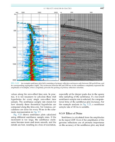
FIG. 9.20 An example semblance plot (left) consisting of primary reflection enclosures only between 300 and 600 ms, and
its corresponding supergather (right). The enclosures between 600 and 2000 ms on the semblance completely represent the
amplitudes of multiples, which completely prevents the picking of primary reflection velocities.

values along the zero-offset time axis. In prac- especially at the deeper parts due to the sparse
tice, it is not necessary to calculate these trial time sampling of the semblance. If a too-small
hyperbolas for every single zero-offset time semblance sample rate is selected, the computa-
sample. The semblance sample rate stands for tional time of the semblance plot increases. For
how densely these theoretical hyperbolas are the example analysis in Fig. 9.23, a semblance
computed along the time axis. For instance, cal- sample rate of 20 ms is suitable.
culations are done for every 50 ms in the sche-
matic representation in Fig. 9.7. 9.3.9 Effect of Noise
Fig. 9.23 shows semblance plots calculated
using different semblance sample rates. If the Semblance is calculated from the amplitudes
increment is too large, the semblance enclo- in the input CDP. Even if the amplitudes of the
sures become more and more smooth, and the genuine reflections are of primary importance
details are lost, resulting in a loss of resolution, on the accuracy of the semblance plot, any kind