Page 455 - Acquisition and Processing of Marine Seismic Data

446 9. VELOCITY ANALYSIS

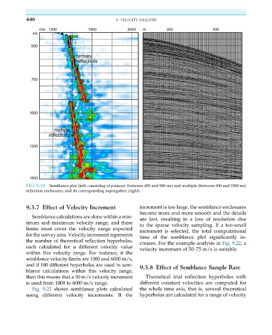
FIG. 9.19 Semblance plot (left) consisting of primary (between 450 and 900 ms) and multiple (between 900 and 1500 ms)
reflection enclosures, and its corresponding supergather (right).

9.3.7 Effect of Velocity Increment increment is too large, the semblance enclosures
become more and more smooth and the details
Semblance calculations are done within a min-
are lost, resulting in a loss of resolution due
imum and maximum velocity range, and these
to the sparse velocity sampling. If a too-small
limits must cover the velocity range expected
increment is selected, the total computational
for the survey area. Velocity increment represents
time of the semblance plot significantly in-
the number of theoretical reflection hyperbolas,
creases. For the example analysis in Fig. 9.22,a
each calculated for a different velocity value velocity increment of 50–75 m/s is suitable.
within this velocity range. For instance, if the
semblance velocity limits are 1000 and 6000 m/s,
and if 100 different hyperbolas are used in sem- 9.3.8 Effect of Semblance Sample Rate
blance calculations within this velocity range,
then this means that a 50 m/s velocity increment Theoretical trial reflection hyperbolas with
is used from 1000 to 6000 m/s range. different constant velocities are computed for
Fig. 9.22 shows semblance plots calculated the whole time axis, that is, several theoretical
using different velocity increments. If the hyperbolas are calculated for a range of velocity