Page 193 - Adaptive Identification and Control of Uncertain Systems with Nonsmooth Dynamics

190 Adaptive Identification and Control of Uncertain Systems with Non-smooth Dynamics

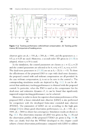
Figure 11.2 Tracking performance with/without compensation. (A) Tracking perfor-
mance; (B) Comparison of tracking errors.

observer gains are β 1 = 100,β 2 = 300,β 3 = 1000, and the parameters γ 1 =
0.5,γ 2 = 0.25 are used. Moreover, a second-order TD given in (11.15)is
adopted, where r 2 = 50 is used.
In the simulation, the control parameters are chosen as c 1 = 12,c 2 = 25
and the control parameters are selected to be θ 1 = θ 2 = 0.7, σ 1 = σ 2 = 0.01.
The dead-zone parameters in (11.55)are setas b r = 25,b l =−15. To show
the effectiveness of the proposed ESO to cope with dead-zone dynamics,
the proposed control with and without compensation are all provided. In
the case without compensation, ξ 3 is set to be zero in the control v.The
corresponding simulation results are depicted in Fig. 11.2. It can be ob-
served that satisfactory tracking performance is obtained with the proposed
control. In particular, when the ESO is used as the compensator for the
dead-zone and unknown dynamics F, it can be found that significantly
improved output tracking performance can be achieved.
Moreover, in order to show the superior observation performance of the
proposed ESO, a linear extended state observer (LESO) is also performed
for comparison with the developed finite-time extended state observer
(FTESO). The parameters of LESO are set according to the high gain
strategy [16] to obtain good observation performance, i.e., β 1 = 100,β 2 =
1500,β 3 = 5800 to obtain fast convergence. Simulation results are shown in
Fig. 11.3. The observation response of LESO was given in Fig. 11.3Aand
the observation profiles of the proposed FTESO are given in Fig. 11.3B.
One can clearly find that the FTESO developed in this chapter could
achieve a better observation performance compared with LESO to address