Page 410 - Advances in Biomechanics and Tissue Regeneration

408 21. NUMERICAL ASSESSMENT OF BONE TISSUE REMODELING

TABLE 21.1 Coefficients of Belinha’s Law
Coefficients j50 j51 j52 j53

a j 0.000E+00 0.000E+00 2.680E+01 2.035E+01
b j 0.000E+00 0.000E+00 2.501E+01 1.247E+00
c j 0.000E+00 7.216E+02 8.059E+02 0.000E+00
d j 1.770E+05 3.861E+05 2.798E+05 6.836E+04
e j 0.000E+00 0.000E+00 2.004E+03 1.442E+02

1 X Q
ρ med ¼ ρ x I (21.10)
ðÞ
Q I¼1
in which Q is the number of integration points and ρ(x I ) the bone apparent density of integration point x I .
The algorithm moves on to the next iterative step, j, performing a new mechanical analysis. It should be noted that a
new material constitutive matrix, c(x I ) j+1 , is constructed for the next iteration given by j+1.
The remodeling process ends when ρ med reaches a value determined by the user or if two consecutive iteration steps
have the same ρ med (Δρ med /Δt=0).

21.3 BONE REMODELING AFTER THA

21.3.1 Computational Model
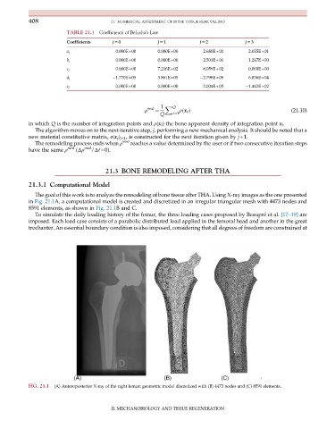
The goal of this work is to analyze the remodeling of bone tissue after THA. Using X-ray images as the one presented
in Fig. 21.1A, a computational model is created and discretized in an irregular triangular mesh with 4473 nodes and
8591 elements, as shown in Fig. 21.1B and C.
To simulate the daily loading history of the femur, the three loading cases proposed by Beaupr e et al. [17–19] are
imposed. Each load case consists of a parabolic distributed load applied in the femoral head and another in the great
trochanter. An essential boundary condition is also imposed, considering that all degrees of freedom are constrained at

FIG. 21.1 (A) Anteroposterior X-ray of the right femur; geometric model discretized with (B) 4473 nodes and (C) 8591 elements.

II. MECHANOBIOLOGY AND TISSUE REGENERATION