Page 218 - Advances in Renewable Energies and Power Technologies

3. Necessity of Joint Adoption of Distributed Maximum Power Point 191

nontracking interval Dt. To evaluate v pk (k ¼ 1, 2, ., N), it is first necessary to
calculate I h ¼ P h /V h , where P h is the power corresponding to V h in the PeV equiv-
alent characteristic of the string of LSCPVUs. Once I h is known, it is then possible to
evaluate v pk (k ¼ 1, 2, ., N) on the basis of the following considerations. In partic-
ular, if I h b I SCk, then v pk ¼ 0; instead, if b I SCk < I h I 0k , then v pk ¼ V cost ;
finally, if I 0k < I h < 0, then v pk ¼ V ds max $I h /(b I SCk ). As an example, let us consider
the case shown in Fig. 5.8 in which the optimal range R b is indeed a single point
V h ¼ 251.9 V. Because it is P h ¼ 767.9 W, therefore I h can be easily evaluated:
I h ¼ P h /V h ¼ 3.05 A. Finally, the values of v pk (k ¼ 1, 2, ., 11) can be obtained
as explained above [23.84, 23.84, 26.34, 26.34, 26.34, 26.34, 0, 0, 0, 0, 0] V. The
same analysis carried out by using the exact PeV characteristic of the string of
LSCPVUs and the exact IeV characteristics of the N LSCPVUs provide instead
the following results: V h ¼ 250.7 V, P h ¼ 781.9 W, I h ¼ 3.119 A, v pk (k ¼ 1, 2,
., 11) ¼ [23.6, 23.6, 27.1, 27.1, 26.2, 26.2, 0, 0, 0, 0, 0] V. The above results clearly
indicate that the suggested procedure is able to provide a quite accurate starting con-
dition for both the DC input inverter voltage and the PV voltages of the LSCPVUs.
The values of such voltages can be successively refined by means of a suitable hill-
climbing technique. In particular, as concerns the DMPPT controllers, in the
following it will be assumed that they carry out an MP&O MPPT technique with
starting conditions v pk (k ¼ 1, 2, ., 11) provided by the FEMPV algorithm. In
the above discussion, it has been assumed that, of course, the inverter is able to oper-
ate at a DC input voltage equal to V h . After the hill climbing refinement step, it is
possible to state that LSCPVUs 1 and 2 will operate at V out ¼ V ds max because of
their high irradiance values; the input operating points of LSCPVUs 3 and 4 will
be their MPPs; LSCPVUs 5 and 6 will operate at a PV voltage slightly lower than
their own V MPP ; and, at last, LSCPVUs 7, 8, 9, 10, and 11 will be short-circuited
because of their low irradiance values. The above statement can be easily explained
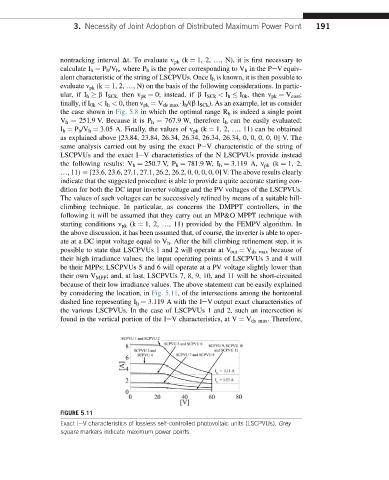
by considering the location, in Fig. 5.11, of the intersections among the horizontal
dashed line representing I h ¼ 3.119 A with the IeV output exact characteristics of
the various LSCPVUs. In the case of LSCPVUs 1 and 2, such an intersection is
found in the vertical portion of the IeV characteristics, at V ¼ V ds max . Therefore,

FIGURE 5.11
Exact IeV characteristics of lossless self-controlled photovoltaic units (LSCPVUs). Grey
square markers indicate maximum power points.