Page 157 - Air Pollution Control Engineering

03_chap_wang.qxd 05/05/2004 12:48 pm Page 136
136 José Renato Coury et al.

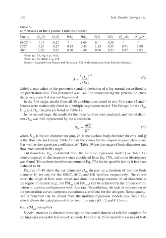
Table 16
Dimensions of the Cyclone Families Studied
Family D /D D /D B/D H/D Z/D S/D H /D D /D
in c e c c c c c cup c cup c
ESCC1 a 0.13 0.24 ? 1.69 0 0.38 ? ?
SCC b 0.24 0.27 0.24 0.45 1.13 0.35 0.71 1.00
GK b 0.20 0.23 0.20 0.40 0.90 0.23 0.87 1.03
a From ref. 53, Fig.5, p. 1416.
b From ref. 56, Table.1, p. 678.
Source: (Adapted from Kenny and Gussman (53), with permission from Elsevier Science.)

σ =  D 16  12 (72)


 D 84 
which is equivalent to the geometric standard deviation of a log-normal curve fitted to
the penetration data. This parameter was used for characterizing the penetration curve
sharpness, even if it was not log-normal.
In the first stage, results from all 36 combinations tested in two flow rates (2 and 4
L/min) were statistically fitted to a multiple-regression model. The fittings for the D ,
50
D , and D (in µm) are listed in Table 17.
16 84
In the second stage, the results for the three families were analyzed, and the cut diam-
eter D was well represented by the correlation:
50
D 50 = aD c b (73)
Q b−1
where D is the cut diameter (in µm), D is the cyclone body diameter (in cm), and Q
50 c
is the flow rate (in L/min). Table 18 lists the values for the empirical parameters a and
2
b as well as the regression coefficient, R . Table 19 lists the range of body diameters and
flow rates tested in this stage.
Cut diameters, D , calculated from the multiple regression model (see Table 17)
50
were compared to the respective ones calculated from Eq. (73), and some discrepancy
was found. The authors therefore recommend Eq. (73) for the specific family it has been
deduced to fit.
Figures 17–19 show the cut diameters D (in µm) as a function of cyclone body
50
diameter D (in cm) for the ESCC, SCC, and GK families, respectively. The curves
c
cover the range of flow rates tested and show that a large number of cut diameters in
the region of interest (e.g., for PM and PM ) can be achieved by the proper combi-
10 2.5
nation of cyclone configuration with flow rate. Nevertheless, the lack of information on
the penetration curves steepness constitutes a problem for the designer. Some qualita-
tive information can be drawn from the multiple-regression models (see Table 17),
which allows the calculation of σ for two flow rates (Q = 2 and 4 L/min).
4.5. PM Samplers
2.5
Special attention is directed nowadays to the establishment of reliable samplers for
the high-risk respirable fraction of aerosols. Peters et al. (57) conducted a series of tests