Page 527 -

INVENTORY SIMULATION 507

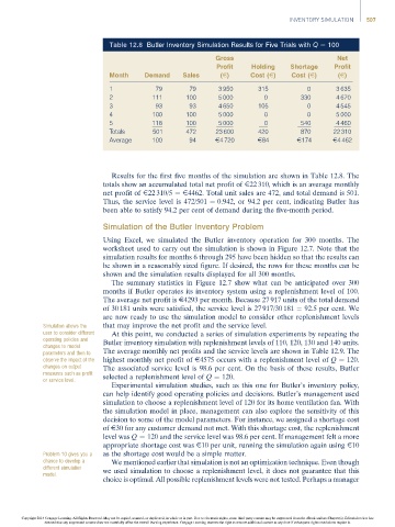
Table 12.8 Butler Inventory Simulation Results for Five Trials with Q ¼ 100
Gross Net
Profit Holding Shortage Profit
Month Demand Sales (E) Cost (E) Cost (E) (E)
1 79 79 3 950 315 0 3 635
2 111 100 5 000 0 330 4 670
3 93 93 4 650 105 0 4 545
4 100 100 5 000 0 0 5 000
5 118 100 5 000 0 540 4 460
Totals 501 472 23 600 420 870 22 310
Average 100 94 E4 720 E84 E174 E4 462

Results for the first five months of the simulation are shown in Table 12.8. The
totals show an accumulated total net profit of E22 310, which is an average monthly
net profit of E22 310/5 ¼ E4462. Total unit sales are 472, and total demand is 501.
Thus, the service level is 472/501 ¼ 0.942, or 94.2 per cent, indicating Butler has
been able to satisfy 94.2 per cent of demand during the five-month period.
Simulation of the Butler Inventory Problem

Using Excel, we simulated the Butler inventory operation for 300 months. The
worksheet used to carry out the simulation is shown in Figure 12.7. Note that the
simulation results for months 6 through 295 have been hidden so that the results can
be shown in a reasonably sized figure. If desired, the rows for these months can be
shown and the simulation results displayed for all 300 months.
The summary statistics in Figure 12.7 show what can be anticipated over 300
months if Butler operates its inventory system using a replenishment level of 100.
The average net profit is E4293 per month. Because 27 917 units of the total demand
of 30 181 units were satisfied, the service level is 27 917/30 181 ¼ 92.5 per cent. We
are now ready to use the simulation model to consider other replenishment levels
Simulation allows the that may improve the net profit and the service level.
user to consider different At this point, we conducted a series of simulation experiments by repeating the
operating policies and
changes to model Butler inventory simulation with replenishment levels of 110, 120, 130 and 140 units.
parameters and then to The average monthly net profits and the service levels are shown in Table 12.9. The
observe the impact of the highest monthly net profit of E4575 occurs with a replenishment level of Q ¼ 120.
changes on output The associated service level is 98.6 per cent. On the basis of these results, Butler
measures such as profit
or service level. selected a replenishment level of Q ¼ 120.
Experimental simulation studies, such as this one for Butler’s inventory policy,
can help identify good operating policies and decisions. Butler’s management used
simulation to choose a replenishment level of 120 for its home ventilation fan. With
the simulation model in place, management can also explore the sensitivity of this
decision to some of the model parameters. For instance, we assigned a shortage cost
of E30 for any customer demand not met. With this shortage cost, the replenishment
level was Q ¼ 120 and the service level was 98.6 per cent. If management felt a more
appropriate shortage cost was E10 per unit, running the simulation again using E10
Problem 10 gives you a as the shortage cost would be a simple matter.
chance to develop a We mentioned earlier that simulation is not an optimization technique. Even though
different simulation we used simulation to choose a replenishment level, it does not guarantee that this
model.
choice is optimal. All possible replenishment levels were not tested. Perhaps a manager

Copyright 2014 Cengage Learning. All Rights Reserved. May not be copied, scanned, or duplicated, in whole or in part. Due to electronic rights, some third party content may be suppressed from the eBook and/or eChapter(s). Editorial review has
deemed that any suppressed content does not materially affect the overall learning experience. Cengage Learning reserves the right to remove additional content at any time if subsequent rights restrictions require it.