Page 530 -

510 CHAPTER 12 SIMULATION

In Chapter 11, we presented formulas that could be used to compute the steady-
state operating characteristics of a queue, including the average waiting time, the
average number of units in the queue, the probability of queuing and so on. In most
cases, the queuing formulas were based on specific assumptions about the proba-
bility distribution for arrivals, the probability distribution for service times, the
queue discipline and so on. Simulation, as an alternative for studying queue, is more
flexible. In applications where the assumptions required by the queuing formulas are
not reasonable, simulation may be the only feasible approach to studying the queu-
ing system. In this section we discuss the simulation of the waiting line for the Hong
Kong Savings Bank automated teller machine (ATM).

Hong Kong Savings Bank ATM Queuing System

Suppose that Hong Kong Savings Bank (HKSB) will open several new branch banks
during the coming year. Each new branch is designed to have one automated teller
machine (ATM). A concern is that during busy periods several customers may have
to wait to use the ATM. This concern prompted the bank to undertake a study of the
ATM queuing system. The bank’s vice president wants to determine whether one
ATM at each branch will be sufficient. The bank established service guidelines for its
ATM system stating that the average customer waiting time for an ATM should be
one minute or less. Let us show how a simulation model can be used to study the
ATM queue at a particular branch.

Customer Arrival Times
One probabilistic input to the ATM simulation model is the arrival times of customers
who use the ATM. In queuing simulations, arrival times are determined by randomly
generating the time between two successive arrivals, referred to as the interarrival time.
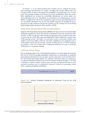
For the branch bank being studied, the customer interarrival times are assumed to
be uniformly distributed between zero and five minutes as shown in Figure 12.8. With
r denoting a random number between zero and one, an interarrival time for two
successive customers can be simulated by using the formula for generating values
from a uniform probability distribution.

Interarrival time ¼ a þ rðb aÞ (12:7)

Figure 12.8 Uniform Probability Distribution of Interarrival Times for the ATM
Queuing System

0 2.5 5
Interarrival Time in Minutes

Copyright 2014 Cengage Learning. All Rights Reserved. May not be copied, scanned, or duplicated, in whole or in part. Due to electronic rights, some third party content may be suppressed from the eBook and/or eChapter(s). Editorial review has
deemed that any suppressed content does not materially affect the overall learning experience. Cengage Learning reserves the right to remove additional content at any time if subsequent rights restrictions require it.