Page 533 -

QUEUING SIMULATION 513

Referring to Figure 12.10, we see that the simulation is initialized in the first block of
the flowchart. Then a new customer arriving is simulated. An interarrival time is
2
generated to determine the time since the preceding customer arrived. The arrival
time for the new customer is then calculated by adding the interarrival time to the
arrival time of the preceding customer.
The decision rule for The arrival time for the new customer must be compared to the completion time
deciding whether the of the preceding customer to determine whether the ATM is idle or busy. If the
ATM is idle or busy is the arrival time of the new customer is greater than the completion time of the preced-
most difficult aspect of
the logic in a queuing ing customer, the preceding customer will have finished service prior to the arrival of
simulation model. the new customer. In this case, the ATM will be idle, and the new customer can
begin service immediately. The service start time for the new customer is equal to
the arrival time of the new customer. However, if the arrival time for the new
customer is not greater than the completion time of the preceding customer, the
new customer arrived before the preceding customer finished service. In this case,
the ATM is busy; the new customer must wait to use the ATM until the preceding
customer completes service. The service start time for the new customer is equal to
the completion time of the preceding customer.
Note that the time the new customer has to wait to use the ATM is the difference
between the customer’s service start time and the customer’s arrival time. At this
point, the customer is ready to use the ATM, and the simulation run continues with
the generation of the customer’s service time. The time at which the customer begins
service plus the service time generated determine the customer’s completion time.
Finally, the total time the customer spends in the system is the difference between
the customer’s service completion time and the customer’s arrival time. At this
point, the computations are complete for the current customer, and the simulation
continues with the next customer. The simulation is continued until a specified
number of customers have been served by the ATM.
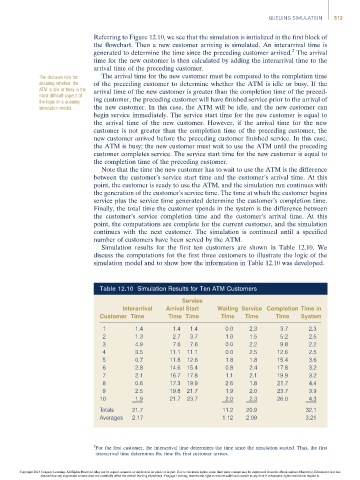
Simulation results for the first ten customers are shown in Table 12.10. We
discuss the computations for the first three customers to illustrate the logic of the
simulation model and to show how the information in Table 12.10 was developed.

Table 12.10 Simulation Results for Ten ATM Customers

Service
Interarrival Arrival Start Waiting Service Completion Time in
Customer Time Time Time Time Time Time System
1 1.4 1.4 1.4 0.0 2.3 3.7 2.3
2 1.3 2.7 3.7 1.0 1.5 5.2 2.5
3 4.9 7.6 7.6 0.0 2.2 9.8 2.2
4 3.5 11.1 11.1 0.0 2.5 12.6 2.5
5 0.7 11.8 12.6 1.8 1.8 15.4 3.6
6 2.8 14.6 15.4 0.8 2.4 17.8 3.2
7 2.1 16.7 17.8 1.1 2.1 19.9 3.2
8 0.6 17.3 19.9 2.6 1.8 21.7 4.4
9 2.5 19.8 21.7 1.9 2.0 23.7 3.9
10 1.9 21.7 23.7 2.0 2.3 26.0 4.3

Totals 21.7 11.2 20.9 32.1
Averages 2.17 1.12 2.09 3.21

2
For the first customer, the interarrival time determines the time since the simulation started. Thus, the first
interarrival time determines the time the first customer arrives.

Copyright 2014 Cengage Learning. All Rights Reserved. May not be copied, scanned, or duplicated, in whole or in part. Due to electronic rights, some third party content may be suppressed from the eBook and/or eChapter(s). Editorial review has
deemed that any suppressed content does not materially affect the overall learning experience. Cengage Learning reserves the right to remove additional content at any time if subsequent rights restrictions require it.