Page 531 -

QUEUING SIMULATION 511

where
r ¼ random number between 0 and 1
a ¼ minimum interarrival time
b ¼ maximum interarrival time
A uniform probability For the HKSB ATM system, the minimum interarrival time is a ¼ zero minutes, and
distribution of interarrival the maximum interarrival time is b ¼ five minutes; therefore, the formula for gen-
times is used here to erating an interarrival time is:
illustrate the simulation
computations. Actually,
any interarrival time
probability distribution Interarrival time ¼ 0 þ rð5 0Þ¼ 5r (12:8)
can be assumed, and the
logic of the waiting line
simulation model will not Assume that the simulation run begins at time ¼ 0 and the first random number of
change. r ¼ 0.2804 generates an interarrival time of 5(0.2804) ¼ 1.4 minutes for customer 1.
Thus, customer 1 arrives 1.4 minutes after the simulation run begins. A second
random number of r ¼ 0.2598 generates an interarrival time of 5(0.2598) ¼ 1.3
minutes, indicating that customer 2 arrives 1.3 minutes after customer 1. Thus,
customer 2 arrives 1.4 þ 1.3 ¼ 2.7 minutes after the simulation begins. Continuing,
a third random number of r ¼ 0.9802 indicates that customer 3 arrives 4.9 minutes
after customer 2, which is 7.6 minutes after the simulation begins.

Customer Service Times
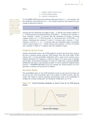
Another probabilistic input in the ATM simulation model is the service time, which is
the time a customer spends using the ATM machine. Past data from similar ATMs
indicate that a normal probability distribution with a mean of two minutes and a
standard deviation of 0.5 minutes, as shown in Figure 12.9, can be used to describe
service times. As discussed in Sections 12.1 and 12.2, values from a normal probability
distribution with mean 2 and standard deviation 0.5 can be generated using the Excel
function ¼ NORMINV(RAND(),2,0.5). For example, the random number of 0.7257
generates a customer service time of 2.3 minutes.
Simulation Model

The probabilistic inputs to the ATM simulation model are the interarrival time and
the service time. The controllable input is the number of ATMs available. The key
results will consist of various operating characteristics such as the probability of
waiting, the average waiting time, the maximum waiting time and so on.

Figure 12.9 Normal Probability Distribution of Service Times for the ATM Queuing
System

Standard Deviation
0.5 Minutes

2
Service Time in Minutes

Copyright 2014 Cengage Learning. All Rights Reserved. May not be copied, scanned, or duplicated, in whole or in part. Due to electronic rights, some third party content may be suppressed from the eBook and/or eChapter(s). Editorial review has
deemed that any suppressed content does not materially affect the overall learning experience. Cengage Learning reserves the right to remove additional content at any time if subsequent rights restrictions require it.