Page 588 -

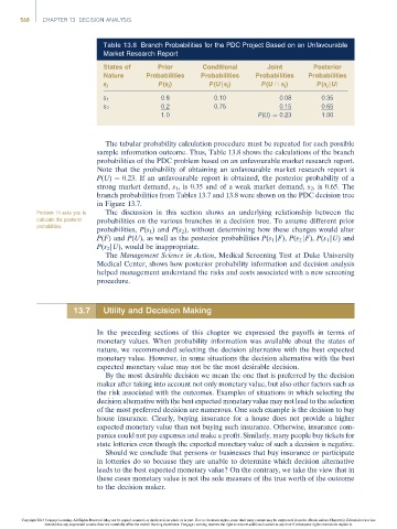
568 CHAPTER 13 DECISION ANALYSIS

Table 13.8 Branch Probabilities for the PDC Project Based on an Unfavourable
Market Research Report
States of Prior Conditional Joint Posterior
Nature Probabilities Probabilities Probabilities Probabilities
P(s j ) P(U|s j ) P(U \ s j ) P(s j |U)
s j
0.8 0.10 0.08 0.35
s 1
0.2 0.75 0.15 0.65
s 2
1.0 P(U) ¼ 0.23 1.00

The tabular probability calculation procedure must be repeated for each possible
sample information outcome. Thus, Table 13.8 shows the calculations of the branch
probabilities of the PDC problem based on an unfavourable market research report.
Note that the probability of obtaining an unfavourable market research report is
P(U) ¼ 0.23. If an unfavourable report is obtained, the posterior probability of a
strong market demand, s 1 , is 0.35 and of a weak market demand, s 2 , is 0.65. The
branch probabilities from Tables 13.7 and 13.8 were shown on the PDC decision tree
in Figure 13.7.
Problem 14 asks you to The discussion in this section shows an underlying relationship between the
calculate the posterior probabilities on the various branches in a decision tree. To assume different prior
probabilities.
probabilities, P(s 1 ) and P(s 2 ), without determining how these changes would alter
P(F) and P(U), as well as the posterior probabilities P(s 1 |F), P(s 2 |F), P(s 1 |U) and
P(s 2 |U), would be inappropriate.
The Management Science in Action, Medical Screening Test at Duke University
Medical Center, shows how posterior probability information and decision analysis
helped management understand the risks and costs associated with a new screening
procedure.

13.7 Utility and Decision Making

In the preceding sections of this chapter we expressed the payoffs in terms of
monetary values. When probability information was available about the states of
nature, we recommended selecting the decision alternative with the best expected
monetary value. However, in some situations the decision alternative with the best
expected monetary value may not be the most desirable decision.
By the most desirable decision we mean the one that is preferred by the decision
maker after taking into account not only monetary value, but also other factors such as
the risk associated with the outcomes. Examples of situations in which selecting the
decision alternative with the best expected monetary value may not lead to the selection
of the most preferred decision are numerous. One such example is the decision to buy
house insurance. Clearly, buying insurance for a house does not provide a higher
expected monetary value than not buying such insurance. Otherwise, insurance com-
panies could not pay expenses and make a profit. Similarly, many people buy tickets for
state lotteries even though the expected monetary value of such a decision is negative.
Should we conclude that persons or businesses that buy insurance or participate
in lotteries do so because they are unable to determine which decision alternative
leads to the best expected monetary value? On the contrary, we take the view that in
these cases monetary value is not the sole measure of the true worth of the outcome
to the decision maker.

Copyright 2014 Cengage Learning. All Rights Reserved. May not be copied, scanned, or duplicated, in whole or in part. Due to electronic rights, some third party content may be suppressed from the eBook and/or eChapter(s). Editorial review has
deemed that any suppressed content does not materially affect the overall learning experience. Cengage Learning reserves the right to remove additional content at any time if subsequent rights restrictions require it.