Page 590 -

570 CHAPTER 13 DECISION ANALYSIS

The three decision alternatives, denoted by d 1 , d 2 and d 3 , are as follows:
d 1 ¼ make investment A
d 2 ¼ make investment B
d 3 ¼ do not invest
The monetary payoffs associated with the investment opportunities depend largely
on what happens to the real estate market during the next six months. Real estate
prices could go up, remain stable or go down. Thus, the states of nature, denoted by
s 1 , s 2 and s 3 , are as follows:

s 1 ¼ real estate prices go up
s 2 ¼ real estate prices remain stable
s 3 ¼ real estate prices go down
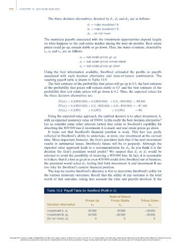
Using the best information available, Swofford estimated the profits or payoffs
associated with each decision alternative and state-of-nature combination. The
resulting payoff table is shown in Table 13.9.
The best estimate of the probability that prices will go up is 0.3, the best estimate
of the probability that prices will remain stable is 0.5 and the best estimate of the
probability that real estate prices will go down is 0.2. Thus, the expected values for
the three decision alternatives are:

EVðd 1 Þ¼ 0:3ðE30 000Þþ 0:5ðE20 000Þþ 0:2ð E50 000Þ¼ E9 000
EVðd 2 Þ¼ 0:3ðE50 000Þþ 0:5ð E20 000Þþ 0:2ð E30 000Þ¼ E1 000
EVðd 3 Þ¼ 0:3ðE0Þ þ 0:5ðE0Þ þ 0:2ðE0Þ ¼ E0
Using the expected value approach, the optimal decision is to select investment A,
with an expected monetary value of E9000. Is this really the best decision alternative?
Let us consider some other relevant factors that relate to Swofford’s capability for
absorbing the E50000 loss if investment A is made and real estate prices go down.
It turns out that Swofford’s financial position is weak. This fact was partly
reflected in Swofford’s ability to undertake, at most, one investment at the current
time. More important, however, the firm’s president feels that if the next investment
results in substantial losses, Swofford’s future will be in jeopardy. Although the
expected value approach leads to a recommendation for d 1 , do you think it is the
decision the firm’s president would prefer? We suspect that d 2 or d 3 would be
selected to avoid the possibility of incurring a E50 000 loss. In fact, it is reasonable
to believe that if a loss as great as even E30 000 could drive Swofford out of business,
the president would select d 3 , feeling that both investment A and investment B are
too risky for Swofford’s current financial position.
The way we resolve Swofford’s dilemma is first to determine Swofford’s utility for
the various monetary outcomes. Recall that the utility of any outcome is the total
worth of that outcome, taking into account the risks and payoffs involved. If the

Table 13.9 Payoff Table for Swofford (Profit in E)

State of Nature
Prices Up Prices Stable Prices Down
Decision Alternative s 1 s 2 s 3
30 000 20 000 50 000
Investment A, d 1
Investment B, d 2 50 000 20 000 30 000
Do not invest, d 3 0 0 0

Copyright 2014 Cengage Learning. All Rights Reserved. May not be copied, scanned, or duplicated, in whole or in part. Due to electronic rights, some third party content may be suppressed from the eBook and/or eChapter(s). Editorial review has
deemed that any suppressed content does not materially affect the overall learning experience. Cengage Learning reserves the right to remove additional content at any time if subsequent rights restrictions require it.