Page 80 -

60 CHAPTER 2 AN INTRODUCTION TO LINEAR PROGRAMMING

convert the constraint to equality form. Just as with slack variables, surplus variables
are given a coefficient of zero in the objective function because they have no effect
on its value. After including two surplus variables, S 1 and S 2 , for the constraints
and one slack variable, S 3 , for the constraint, the linear programming model of
the M&D Chemicals problem becomes:
Min 2A þ 3B þ 0S 1 þ 0S 2 þ 0S 3
s:t:
1A 1S 1 ¼ 125
1A þ 1B 1S 2 ¼ 350
2A þ 1B þ 1S 3 ¼ 600
A; B; S 1 ; S 2 ; S 3 0
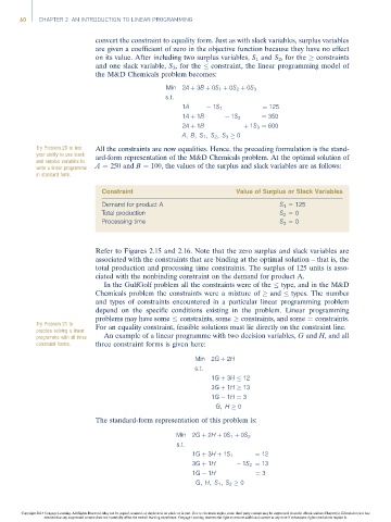
Try Problem 20 to test All the constraints are now equalities. Hence, the preceding formulation is the stand-
your ability to use slack ard-form representation of the M&D Chemicals problem. At the optimal solution of
and surplus variables to
write a linear programme A ¼ 250 and B ¼ 100, the values of the surplus and slack variables are as follows:
in standard form.

Constraint Value of Surplus or Slack Variables
Demand for product A S 1 = 125
Total production S 2 =0
Processing time S 3 =0

Refer to Figures 2.15 and 2.16. Note that the zero surplus and slack variables are
associated with the constraints that are binding at the optimal solution – that is, the
total production and processing time constraints. The surplus of 125 units is asso-
ciated with the nonbinding constraint on the demand for product A.
In the GulfGolf problem all the constraints were of the type, and in the M&D
Chemicals problem the constraints were a mixture of and types. The number
and types of constraints encountered in a particular linear programming problem
depend on the specific conditions existing in the problem. Linear programming
problems may have some constraints, some constraints, and some ¼ constraints.
Try Problem 21 to
practice solving a linear For an equality constraint, feasible solutions must lie directly on the constraint line.
programme with all three An example of a linear programme with two decision variables, G and H, and all
constraint forms. three constraint forms is given here:
Min 2G þ 2H
s:t:
1G þ 3H 12
3G þ 1H 13
1G 1H ¼ 3
G; H 0
The standard-form representation of this problem is:

Min 2G þ 2H þ 0S 1 þ 0S 2
s:t:
1G þ 3H þ 1S 1 ¼ 12
3G þ 1H 1S 2 ¼ 13
1G 1H ¼ 3
G; H; S 1 ; S 2 0

Copyright 2014 Cengage Learning. All Rights Reserved. May not be copied, scanned, or duplicated, in whole or in part. Due to electronic rights, some third party content may be suppressed from the eBook and/or eChapter(s). Editorial review has
deemed that any suppressed content does not materially affect the overall learning experience. Cengage Learning reserves the right to remove additional content at any time if subsequent rights restrictions require it.