Page 124 - Analog and Digital Filter Design

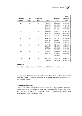
121
Poles and Zeroes

Pole
Stopband Filter Attenuation Pole Real Imaginary
Frequency Order (dB) Zero Part Part

1.1 8 59 3.886673 0.2486642 0.3003527
1.542858 0.1396883 0.73 77445
I. 1946 I4 0.0547358 0.9343149
I . I08280 0.01 33884 0.9992589
I .1 6 so 3.598981 0.289467 3 0.3598184
1.495323 0. 1365805 0.8342558
1.227 I6 0.0332612 0.9983043

1 .3 6 57 4,130155 0.2757091 0.3356090
1.664290 0.1454597 0.8107855
1.328862 0.0390806 0.9974829

I .4 6 63 4.618428 0.2669266 0.3208161
1.825298 0. I508535 0.7950983
I .-I31274 0.043 I288 0.9968596
I .5 5 53 2.331876 0.2288748 0.68 167s I
1.557406 0.0665407 0.9952537
0.3378465
2.0 4 51 4.922 1 13 0.35 12734 0.4424978
2.143 I89 0. I214786 0.989 I762

Table 3.30
Cauer Pole and Zero Locations (1dB Ripple and 50dB Stopband Attenuation)

In some cases the values given in one table are the same as another. This occurs
when the stopband attenuation achieved in producing one table exceeds that
required for the next.

Cauer Pole Zero Plot
Cauer filters have a pole pattern similar to that of Chebyshev filters. The poles
are placed in an elliptical pattern, but Cauer filters also have zeroes on the iniag-
inary axis. An example of this is given in Figure 3.13, which shows the pole zero
diagram for a fifth-order Cauer filter.