Page 141 - Analog and Digital Filter Design

1 38 Analog and Digital Filter Design

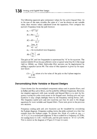
The following equations give component values for the active biquad filter. As
in the case of the state variable, the value of C can be chosen as any suitable
value, then resistor values calculated from the equations. First compute the
section’s frequency from the pole location:
a,, =JGGz
1
R1= R4 = -
20 c
1
R2 = R3 = -
0, c
200,, R
R5=-
w> -a,;
cor = the normalized zero frequency.

The gain at DC and low frequencies is represented by “A” in the equation. The
resistors labeled R can be any arbitrary value; a typical value may be in the range
1 kS2 to 100kQ say 10kQ. Odd-order filter sections can be implemented by
adding a capacitor across R6. The value of this capacitor is given by the equa-
tion below:
1
C6 = - where Q is the value of the pole on the S-plane negative
B R6
real axis.

Denormalizing State Variable or Biquad Designs

I have shown that the normalized component values used in passive filters, and
in Sallen and Key active filters, can be scaled for different frequencies. However,
the simplest approach with state variable and biquad filters is to start by fre-
quency scaling the poles (and zeroes in the biquad case). Scaling pole and zero
locations is easy: simply multiply them by the frequency scaling factor, 27rFc,.
The frequency scaled pole and zero locations can then be used in the design
equations for state variable and biquad filters. These were given in the previous
two sections.

Frequency scaling pole and zero locations can be visualized by considering
the S-plane diagram. Frequency scaling moves the poles outward on a line that
extends from the S-plane origin. To picture this, think of a pole at, say, s =
-0.75 + j 1.2 in a normalized response. If this is scaled for a frequency of 10Hz,
the scaling factor is 2 nFc = 62.83 rad/s, and the pole moves to -47.12 + j75.396.
This is shown in the diagram of Figure 4.14 (not to scale).