Page 142 - Analog and Digital Filter Design

139
Analog Lowpass Filters

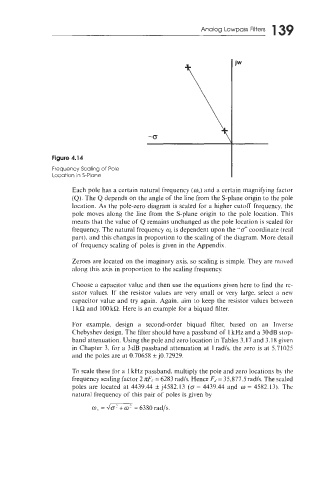
Figure 4.14
Frequency Scaling of Pole
Location in S-Plane

Each pole has a certain natural frequency (m,,) and a certain magnifying factor
(Q). The Q depends on the angle of the line from the S-plane origin to the pole
location. As the pole-zero diagram is scaled for a higher cutoff frequency. the
pole moves along the line from the S-plane origin to the pole location. This
means that the value of Q remains unchanged as the pole location is scaled for
frequency. The natural frequency w,, is dependent upon the "o" coordinate (real
part), and this changes in proportion to the scaling of the diagram. More detail
of frequency scaling of poles is given in the Appendix.

Zeroes are located on the imaginary axis. so scaling is simple. They are moved
along this axis in proportion to the scaling frequency.

Choose a capacitor value and then use the equations given here to find the re-
sistor values. If the resistor values are very small or very large. select a new
capacitor value and try again. Again. aim to keep the resistor values between
1 kR and 100 kR. Here is an example for a biquad filter.
For example, design a second-order biquad filter, based on an Inverse
Chebyshev design. The filter should have a passband of 1 kHz and a 30dB stop-
band attenuation. Using the pole and zero location in Tables 3.17 and 3.18 given
in Chapter 3, for a 3dB passband attenuation at 1 rad/s. the zero is at 5.71025
and the poles are at 0.70658 f j0.72929.

To scale these for a 1 kHz passband, multiply the pole and zero locations by the
frequency scaling factor 2 nFc = 6283 radls. Hence FL = 35.877.5 radls. The scaled
poles are located at 4439.44 f j4582.13 (CT = 4439.44 and w = 4582.13). The
natural frequency of this pair of poles is given by
w,, = do' +w' = 6380 rad/s.