Page 215 - Analog and Digital Filter Design

2 1 2 Analog and Digital Filter Design

The frequencies are fR, = f. = 44.59091 and fR2 = rVfo = 55.835493.
w
w
The pole’s Q factor is given by Q = - 13.1206264.
=
A+h
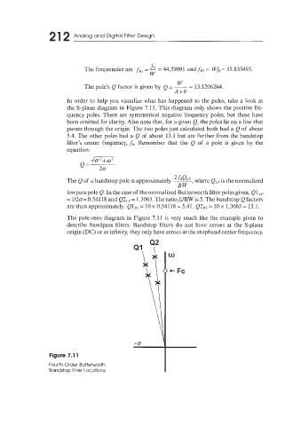
In order to help you visualize what has happened to the poles, take a look at
the S-plane diagram in Figure 7.11. This diagram only shows the positive fre-
quency poles. There are symmetrical negative frequency poles, but these have
been omitted for clarity. Also note that, for a given Q, the poles lie on a line that
passes through the origin. The two poles just calculated both had a Q of about
5.4. The other poles had a Q of about 13.1 but are further from the bandstop
filter’s center frequency, fo. Remember that the Q of a pole is given by the
equation:
JzTz

20

The Q of a bandstop pole is approximately ~ 2hQLp, where QLP is the normalized
B LT’
lowpass pole Q. In the case of the normalized Butterworth filter poles given, elLp
= 1/20=0.54118 and Q2Lp= 1.3065. TheratiojJBW is 5. The bandstop Qfactors
are thenapproximately: elBs= lOx0.54118=5.41. Q2ss= lox 1.3065= 13.1.

The pole-zero diagram in Figure 7.11 is very much like the example given to
describe bandpass filters. Bandstop filters do not have zeroes at the S-plane
origin (DC) or at infinity, they only have zeroes at the stopband center frequency.
Q1 ?*

Figure 7.1 1
Fourth-Order Butterworth
Bandstop Pole Locations