Page 74 - Analog and Digital Filter Design

7 1
Time and Frequency Response

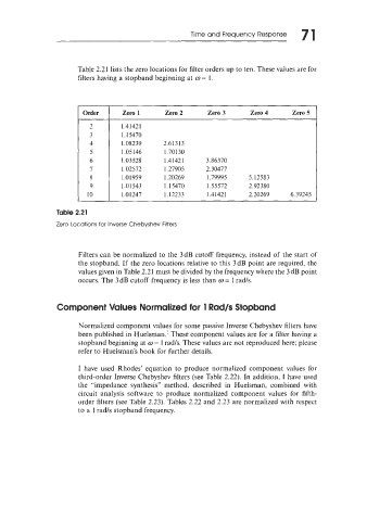
Table 2.21 lists the zero locations for filter orders up to ten. These values are for
filters having a stopband beginning at w = 1.

Order Zero 1 Zero 2 Zero 3 Zero 4 Zero 5

7 1.41421
1.15470
4 1.08239 2.61313
5 1.05146 1.70130
6 1.03528 1.4 142 1 3.86370
7 1.02572 1.27905 2.30477
8 1.01959 1.20269 1.79995 5.12583
9 1 .O 1543 I. I5470 1.55572 2.92380
10 1.01247 1.12233 1.41421 2.20269 6.39245
~~
Table 2.21

Zero Locations for Inverse Chebyshev Filters

Filters can be normalized to the 3dB cutoff frequency, instead of the start of
the stopband. If the zero locations relative to this 3dB point are required, the
values given in Table 2.21 must be divided by the frequency where the 3 dB point
occurs. The 3 dB cutoff frequency is less than w = 1 rad/s.

Component Values Normalized for 1 Rad/s Stopband

Normalized component values for some passive Inverse Chebyshev filters have
been published in Huelsman.’ These component values are for a filter having a
stopband beginning at w = 1 radls. These values are not reproduced here; please
refer to Huelsman’s book for further details.

I have used Rhodes’ equation to produce normalized component values for
third-order Inverse Chebyshev filters (see Table 2.22). In addition, I have used
the “impedance synthesis” method, described in Huelsman, combined with
circuit analysis software to produce normalized component values for fifth-
order filters (see Table 2.23). Tables 2.22 and 2.23 are normalized with respect
to a 1 rads stopband frequency.