Page 54 - Analytical Electrochemistry 2d Ed - Jospeh Wang

2-1 CYCLIC VOLTAMMETRY 39

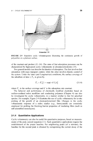
FIGURE 2-9 Repetitive cyclic voltammograms illustrating the continuous growth of
polyaniline on a platinum surface.

of the reactant and product (11±14). The rates of fast adsorption processes can be
characterized by high-speed cyclic voltammetry at ultramicroelectrodes (15).
Two general models can describe the kinetics of adsorption. The ®rst involves fast
adsorption with mass transport control, while the other involves kinetic control of
the system. Under the latter (and Langmuirian) conditions, the surface coverage of
the adsorbate at time t, G , is given by.
t

0
G ˆ G 1 exp k C t† 2-14†
t
e
t
where G is the surface coverage and k is the adsorption rate constant.
0
e
The behavior and performance of chemically modi®ed electrodes based on
surface-con®ned redox modi®ers and conducting polymers (Chapter 4) can also
be investigated by cyclic voltammetry, in a manner similar to that for adsorbed
species. For example, Figure 2-9 illustrates the use of cyclic voltammetry for in-situ
probing of the growth of an electropolymerized ®lm. Changes in the cyclic
voltammetric response of a redox marker (e.g., ferrocyanide) are commonly
employed for probing the blocking=barrier properties of insulating ®lms (such as
self-assembled monolayers).

2-1.4 Quantitative Applications
Cyclic voltammetry can also be useful for quantitative purposes, based on measure-
ments of the peak current (equation 2-1). Such quantitative applications require the
establishment of the proper baseline. For neighboring peaks (of a mixture), the
baseline for the second peak is obtained by extrapolating the current decay of the