Page 84 - Analytical Electrochemistry 2d Ed - Jospeh Wang

3-3 PULSE VOLTAMMETRY 69

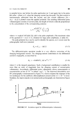
is sampled twice, just before the pulse application (at 1) and again late in the pulse
life (after 40 ms, at 2, when the charging current has decayed). The ®rst current is
instrumentally subtracted from the second, and this current difference ‰Di ˆ
i t † i t †Š is plotted versus the applied potential. The resulting differential pulse
2
1
voltammogram consists of current peaks, the height of which is directly proportional
to the concentration of the corresponding analytes:
nFAD 1=2 C 1 s
i ˆ p  3-16†
p
pt m 1 ‡ s
where s ˆ exp‰ nF=RT† DE=2†Š.(DE is the pulse amplitude.) The maximum value
of the quotient 1 s†= 1 ‡ s†, obtained for large pulse amplitudes, is unity (6).
The peak potential E † can be used to identify the species, as it occurs near the
p
polarographic half-wave potential:

E ˆ E DE=2 3-17†
p 1=2

The differential-pulse operation results in a very effective correction of the
charging background current. The charging-current contribution to the differential
current is negligible, as described by

Di ' 0:00567C DEm 2=3 1=3 3-18†
t
c
i
where C is the integral capacitance. Such a background contribution is smaller by
i
more than an order of magnitude than the charging current of normal-pulse
voltammetry. Accordingly, differential pulse voltammetry allows measurements at
1
concentrations as low as 10 8 M (about 1 mgL ). The improved detectability over
DC polarography is demonstrated in Figure 3-6, which compares the response of the
two techniques for the antibiotic chloramphenicol present at the 1:3 10 5 M level.
Similarly, the improvements over normal-pulse polarography are illustrated in Figure
3-7.

FIGURE 3-5 Excitation signal for differential-pulse voltammetry.