Page 469 - Applied Numerical Methods Using MATLAB

458 PARTIAL DIFFERENTIAL EQUATIONS
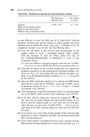
Table P9.8.3 The Maximum Absolute Error and the Number of Nodes
The Maximum The Number
Absolute Error of Nodes

poisson() 7.5462 × 10 −4 41 × 101
PDEtool with Initialize Mesh
PDEtool with Refine Mesh
PDEtool with second Refine Mesh

use the PDEtool to solve this PDE and fill in Table P9.8.3 with the
maximum absolute error and the number of nodes together with those
obtained with the MATLAB routine ‘heat_CN()’ in Problem 9.4(c) for
comparison. In order to do this job, take the following steps.
(1) Click the button in the tool-bar and click-and-drag on the
graphic region to create a rectangular domain. Then, double-
click the rectangle to open the Object dialog box and set
the Left/Bottom/Width/Height to 0/0/pi/0.01 to make a long
rectangular domain.
(cf) Even if the PDEtool is originally designed to deal with only 2-D PDEs,
we can use it to solve 1-D PDEs like (P9.8.8) by proceeding in this way.
(2) Click the ∂ button in the tool-bar, double-click the upper/lower
boundary segments to set the homogeneous Neumann boundary con-
dition (g = 0, q = 0) and double-click the left/right boundary seg-
ments to set the Dirichlet boundary condition (h = 1, r = 0) as given
by Eq. (P9.8.9).
(3) Open the PDE specification dialog box by clicking the PDE button,
check the box on the left of ‘Parabolic’ as the type of PDE, and set
its parameters in Eq. (9.5.5) as c = 2, a = 0, f = 0and d = 1, which
corresponds to Eq. (P9.8.8).
(4) Click ‘Parameters’ in the Solve pull-down menu to set the time range,
say, as 0:0.002:0.2 and to set the initial conditions as Eq. (P9.8.9).
(5) In the Plot selection dialog box opened by clicking the but-
ton, check the box before Height and click the Plot button. If you
want to plot the solution graph at a time other than the final time,
select the time for plot from {0, 0.002, 0.004,..., 0.2} in the far-
right field of the Plot selection dialog box and click the Plot but-
ton again.
(6) If you want to see a movie-like dynamic picture of the solution graph,
check the box before Animation and then click the Plot button in the
Plot selection dialog box.
(7) Click ‘Export Mesh’ in the Mesh pull-down menu, and then click the
OK button in the Export dialog box to extract the mesh data {p,e,t }.