Page 470 - Applied Numerical Methods Using MATLAB

PROBLEMS 459
Also click ‘Export Solution’ in the Solve pull-down menu, and then
click the OK button in the Export dialog box to extract the solution
u. Now, you can estimate how far the graphical/numerical solution
deviates from the true solution (P9.8.10) by typing the following
statements into the MATLAB command window:

>>x = p(1,:)’; y = p(2,: )’; %x,y coordinates of nodes in columns
>>tt = 0:0.01:0.2; %time vector in row
>>err = sin(2*x)*exp(-8*tt)-u; %deviation from true sol.(P9.8-10)
>>err_max = max(abs(err)) %maximum absolute error

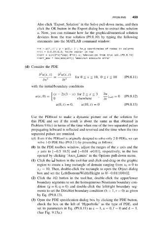
(d) Consider the PDE

2
2
∂ u(x, t) ∂ u(x, t)
= for 0 ≤ x ≤ 10, 0 ≤ t ≤ 10 (P9.8.11)
∂x 2 ∂t 2
with the initial/boundary conditions

(x − 2)(3 − x) for 2 ≤ x ≤ 3 ∂u
u(x, 0) = , | t=0 = 0 (P9.8.12)
0 elsewhere ∂t
u(0,t) = 0, u(10,t) = 0 (P9.8.13)

Use the PDEtool to make a dynamic picture out of the solution for
this PDE and see if the result is about the same as that obtained in
Problem 9.6(c) in terms of the time when one of the two separated pulses
propagating leftward is reflected and reversed and the time when the two
separated pulses are reunited.
(cf) Even if the PDEtool is originally designed to solve only 2-D PDEs, we can
solve 1-D PDE like (P9.8.11) by proceeding as follows:
(0) In the PDE toolbox window, adjust the ranges of the x axis and the
y axis to [−0.5 10.5] and [−0.01 +0.01], respectively, in the box
opened by clicking ‘Axes Limits’ in the Options pull-down menu.
(1) Click the button in the tool-bar and click-and-drag on the graphic
region to create a long rectangle of domain ranging from x 0 = 0to
x f = 10. Then, double-click the rectangle to open the Object dialog
box and set the Left/Bottom/Width/Height to 0/−0.01/10/0.02.
(2) Click the ∂ button in the tool-bar, double-click the upper/lower
boundary segments to set the homogeneous Neumann boundary con-
dition (g = 0, q = 0) and double-click the left/right boundary seg-
ments to set the Dirichlet boundary condition (h = 1, r = 0) as given
by Eq. (P9.8.13).
(3) Open the PDE specification dialog box by clicking the PDE button,
check the box on the left of ‘Hyperbolic’ as the type of PDE, and
set its parameters in Eq. (P9.8.11) as c = 1, a = 0, f = 0andd = 1.
(See Fig. 9.15a.)