Page 368 - Applied Statistics And Probability For Engineers

c09.qxd 5/15/02 8:02 PM Page 316 RK UL 9 RK UL 9:Desktop Folder:

316 CHAPTER 9 TESTS OF HYPOTHESES FOR A SINGLE SAMPLE

The test procedure requires a random sample of size n from the population whose proba-
bility distribution is unknown. These n observations are arranged in a frequency histogram,
having k bins or class intervals. Let O be the observed frequency in the ith class interval. From
i
the hypothesized probability distribution, we compute the expected frequency in the ith class
interval, denoted E i . The test statistic is

k 1O
E 2 2
2
X a i i (9-39)
0
i 1 E i

It can be shown that, if the population follows the hypothesized distribution, X 2 0 has, approx-
imately, a chi-square distribution with k
p
1 degrees of freedom, where p represents the
number of parameters of the hypothesized distribution estimated by sample statistics. This ap-
proximation improves as n increases. We would reject the hypothesis that the distribution of
the population is the hypothesized distribution if the calculated value of the test statistic
2
2 ,k
p
1 .
0
One point to be noted in the application of this test procedure concerns the magnitude
of the expected frequencies. If these expected frequencies are too small, the test statistic X 0 2
will not reflect the departure of observed from expected, but only the small magnitude of
the expected frequencies. There is no general agreement regarding the minimum value of
expected frequencies, but values of 3, 4, and 5 are widely used as minimal. Some writers
suggest that an expected frequency could be as small as 1 or 2, so long as most of them ex-
ceed 5. Should an expected frequency be too small, it can be combined with the expected
frequency in an adjacent class interval. The corresponding observed frequencies would then
also be combined, and k would be reduced by 1. Class intervals are not required to be of
equal width.
We now give two examples of the test procedure.

EXAMPLE 9-12 A Poisson Distribution
The number of defects in printed circuit boards is hypothesized to follow a Poisson distribu-
tion. A random sample of n 60 printed boards has been collected, and the following num-
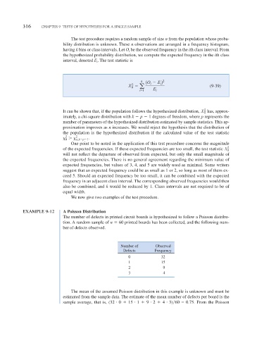
ber of defects observed.

Number of Observed
Defects Frequency
0 32
1 15
2 9
3 4

The mean of the assumed Poisson distribution in this example is unknown and must be
estimated from the sample data. The estimate of the mean number of defects per board is the
sample average, that is, (32 0 15 1 9 2 4 3) 60 0.75. From the Poisson