Page 370 - Applied Statistics And Probability For Engineers

c09.qxd 5/15/02 8:02 PM Page 318 RK UL 9 RK UL 9:Desktop Folder:

318 CHAPTER 9 TESTS OF HYPOTHESES FOR A SINGLE SAMPLE

2
2
6. Reject H if 0.05,1 3.84.
0
0
7. Computations:
2 2 2
132
28.322 115
21.242 113
10.442
2
0 2.94
28.32 21.24 10.44
2 2.94 2
8. Conclusions: Since 0 0.05,1 3.84, we are unable to reject the null hypothesis
that the distribution of defects in printed circuit boards is Poisson. The P-value for the
test is P 0.0864. (This value was computed using an HP-48 calculator.)
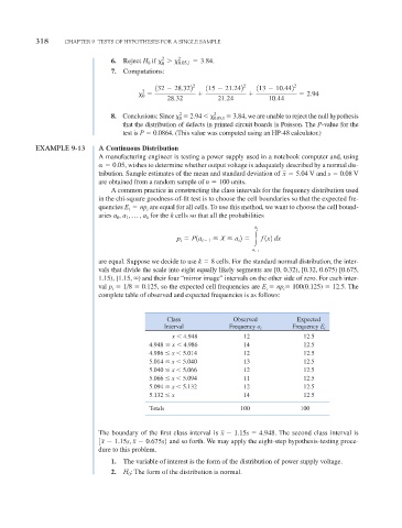
EXAMPLE 9-13 A Continuous Distribution
A manufacturing engineer is testing a power supply used in a notebook computer and, using
0.05, wishes to determine whether output voltage is adequately described by a normal dis-
tribution. Sample estimates of the mean and standard deviation of x 5.04 V and s 0.08 V
are obtained from a random sample of n 100 units.
A common practice in constructing the class intervals for the frequency distribution used
in the chi-square goodness-of-fit test is to choose the cell boundaries so that the expected fre-
np are equal for all cells. To use this method, we want to choose the cell bound-
quencies E i i
aries a , a , p , a for the k cells so that all the probabilities
1
k
0
a i
p P1a i
1 X a 2 f 1x2 dx
i
i
a i
1
are equal. Suppose we decide to use k 8 cells. For the standard normal distribution, the inter-
vals that divide the scale into eight equally likely segments are [0, 0.32), [0.32, 0.675) [0.675,
1.15), [1.15, ) and their four “mirror image” intervals on the other side of zero. For each inter-
val p 1 8 0.125, so the expected cell frequencies are E np 100(0.125) 12.5. The
i
i
i
complete table of observed and expected frequencies is as follows:
Class Observed Expected
Interval Frequency o i Frequency E i
x 4.948 12 12.5
4.948 x 4.986 14 12.5
4.986 x 5.014 12 12.5
5.014 x 5.040 13 12.5
5.040 x 5.066 12 12.5
5.066 x 5.094 11 12.5
5.094 x 5.132 12 12.5
5.132 x 14 12.5

Totals 100 100

The boundary of the first class interval is x
1.15s 4.948 . The second class interval is
3x
1.15s, x
0.675s2 and so forth. We may apply the eight-step hypothesis-testing proce-
dure to this problem.
1. The variable of interest is the form of the distribution of power supply voltage.
2. H : The form of the distribution is normal.
0