Page 369 - Applied Statistics And Probability For Engineers

c09.qxd 5/15/02 8:02 PM Page 317 RK UL 9 RK UL 9:Desktop Folder:

9-7 TESTING FOR GOODNESS OF FIT 317

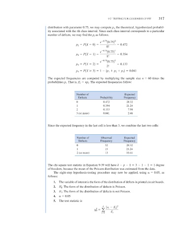
distribution with parameter 0.75, we may compute p i , the theoretical, hypothesized probabil-
ity associated with the ith class interval. Since each class interval corresponds to a particular
number of defects, we may find the p as follows:
i
e
0.75 10.752 0
p P1X 02 0.472
1
0!
e
0.75 10.752 1
p P1X 12 0.354
2
1!
e
0.75 10.752 2
p P1X 22 0.133
3
2!
p P1X 32 1
1p 1 p 2 p 3 2 0.041
4
The expected frequencies are computed by multiplying the sample size n 60 times the
probabilities p . That is, E i np i . The expected frequencies follow:
i

Number of Expected
Defects Probability Frequency
0 0.472 28.32
1 0.354 21.24
2 0.133 7.98
3 (or more) 0.041 2.46

Since the expected frequency in the last cell is less than 3, we combine the last two cells:

Number of Observed Expected
Defects Frequency Frequency
0 32 28.32
1 15 21.24
2 (or more) 13 10.44

The chi-square test statistic in Equation 9-39 will have k
p
1 3
1
1 1 degree
of freedom, because the mean of the Poisson distribution was estimated from the data.
The eight-step hypothesis-testing procedure may now be applied, using 0.05, as
follows:
1. The variable of interest is the form of the distribution of defects in printed circuit boards.
2. H : The form of the distribution of defects is Poisson.
0
3. H : The form of the distribution of defects is not Poisson.
1
4. 0.05
5. The test statistic is
k 1o i
E i 2 2
2
0 a
i 1 E i