Page 400 - Applied Statistics And Probability For Engineers

c10.qxd 5/16/02 1:31 PM Page 344 RK UL 6 RK UL 6:Desktop Folder:TEMP WORK:MONTGOMERY:REVISES UPLO D CH114 FIN L:Quark Files:

344 CHAPTER 10 STATISTICAL INFERENCE FOR TWO SAMPLES

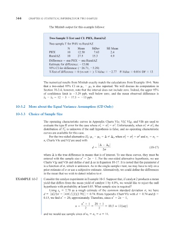
The Minitab output for this example follows:

Two-Sample T-Test and CI: PHX, RuralAZ
Two-sample T for PHX vs RuralAZ
N Mean StDev SE Mean
PHX 10 12.50 7.63 2.4
RuralAZ 10 27.5 15.3 4.9
Difference mu PHX mu RuralAZ
Estimate for difference: 15.00
95% CI for difference: ( 26.71, 3.29)
T-Test of difference 0 (vs not ): T-Value 2.77 P-Value 0.016 DF 13

The numerical results from Minitab exactly match the calculations from Example 10-6. Note
that a two-sided 95% CI on 1 2 is also reported. We will discuss its computation in
Section 10-3.4; however, note that the interval does not include zero. Indeed, the upper 95%
of confidence limit is 3.29 ppb, well below zero, and the mean observed difference is
x x 12 5 17.5 15 ppb .
1
2
10-3.2 More about the Equal Variance Assumption (CD Only)

10-3.3 Choice of Sample Size

The operating characteristic curves in Appendix Charts VIe, VIf, VIg, and VIh are used to
2
2
2
2
2
evaluate the type II error for the case where . Unfortunately, when , the
1
1
2
2
*
distribution of T 0 is unknown if the null hypothesis is false, and no operating characteristic
curves are available for this case.
2
2
2
For the two-sided alternative H 1 : 1 2 0 , when and n 1 n 2
1
2
n, Charts VIe and VIf are used with
ƒ ƒ
0
d (10-17)
2
where is the true difference in means that is of interest. To use these curves, they must be
entered with the sample size n * 2n 1. For the one-sided alternative hypothesis, we use
Charts VIg and VIh and define d and as in Equation 10-17. It is noted that the parameter d
is a function of , which is unknown. As in the single-sample t-test, we may have to rely on a
prior estimate of or use a subjective estimate. Alternatively, we could define the differences
in the mean that we wish to detect relative to .
EXAMPLE 10-7 Consider the catalyst experiment in Example 10-5. Suppose that, if catalyst 2 produces a mean
yield that differs from the mean yield of catalyst 1 by 4.0%, we would like to reject the null
hypothesis with probability at least 0.85. What sample size is required?
Using s p 2.70 as a rough estimate of the common standard deviation , we have
d ƒ ƒ
2 ƒ 4.0 ƒ
312212.7024 0.74. From Appendix Chart VIe with d 0.74 and
*
*
0.15, we find n 20, approximately. Therefore, since n 2n 1,
*
n 1 20 1
n 10.5 111say2
2 2
and we would use sample sizes of n 1 n 2 n 11.