Page 179 - Applied statistics and probability for engineers

Section 5-1/Two or More Random Variables 157

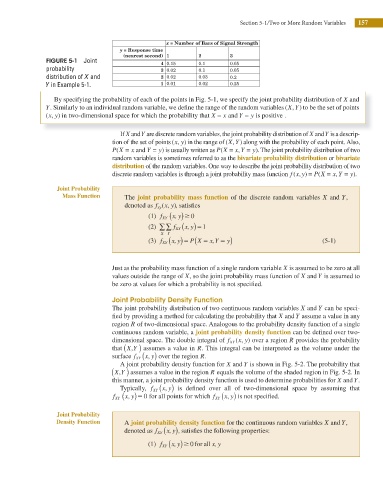
x = Number of Bars of Signal Strength
y = Response time
(nearest second) 1 2 3
FIGURE 5-1 Joint
4 0.15 0.1 0.05
probability 3 0.02 0.1 0.05
distribution of X and 2 0.02 0.03 0.2
Y in Example 5-1. 1 0.01 0.02 0.25

By specifying the probability of each of the points in Fig. 5-1, we specify the joint probability distribution of X and
Y
Y. Similarly to an individual random variable, we deine the range of the random variables ( , ) to be the set of points
X

( , ) in two-dimensional space for which the probability that X = x and Y = y is positive .
x
y
If X and Y are discrete random variables, the joint probability distribution of X and Y is a descrip-
X
Y
tion of the set of points ( , ) in the range of ( , ) along with the probability of each point. Also,
y
x
(
(
P X = x and Y = y ) is usually written as P X = x Y = y). The joint probability distribution of two
,
random variables is sometimes referred to as the bivariate probability distribution or bivariate
distribution of the random variables. One way to describe the joint probability distribution of two
discrete random variables is through a joint probability mass function f x y( , ) = P X = x Y = y).
(
,
Joint Probability
Mass Function The joint probability mass function of the discrete random variables X and Y,
denoted as f xy ( x y), satisi es
,
(1) f XY ( x, y)$ 0

(2) ∑ ∑ f XY ( x, y)51

X Y
(3) f XY ( x, y)5 P X ( 5 x,Y 5 y) (5-1)

Just as the probability mass function of a single random variable X is assumed to be zero at all
values outside the range of X, so the joint probability mass function of X and Y is assumed to
be zero at values for which a probability is not specii ed.
Joint Probability Density Function
The joint probability distribution of two continuous random variables X and Y can be speci-

ied by providing a method for calculating the probability that X and Y assume a value in any
region R of two-dimensional space. Analogous to the probability density function of a single
continuous random variable, a joint probability density function can be dei ned over two-
,
dimensional space. The double integral of f XY ( x y) over a region R provides the probability
, (
that X Y ) assumes a value in R. This integral can be interpreted as the volume under the
surface f XY ( x y) over the region R.

,
A joint probability density function for X and Y is shown in Fig. 5-2. The probability that
, (
X Y ) assumes a value in the region R equals the volume of the shaded region in Fig. 5-2. In
this manner, a joint probability density function is used to determine probabilities for X and Y.
Typically, f XY ( x y) is dei ned over all of two-dimensional space by assuming that

,
f XY ( x y)50 for all points for which f XY ( x y) is not specii ed.

,
,
Joint Probability
Density Function A joint probability density function for the continuous random variables X and Y,
denoted as f XY ( x, y , ) satisies the following properties:

(1) f XY ( x, y) $ 0 for all x, y