Page 181 - Applied statistics and probability for engineers

Section 5-1/Two or More Random Variables 159

y y

2000

0
0 x 0 1000 x
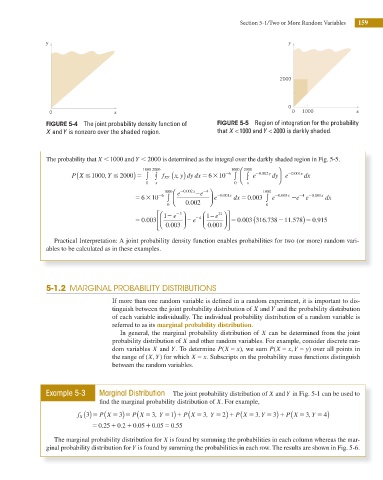
FIGURE 5-4 The joint probability density function of FIGURE 5-5 Region of integration for the probability
X and Y is nonzero over the shaded region. that X <1000 and Y < 2000 is darkly shaded.

The probability that X ,1000 and Y , 2000 is determined as the integral over the darkly shaded region in Fig. 5-5.

(
)
∫
∫
∫
0 001
.
P X #1000 ,Y # 2000) 5 1000 2000 f XY ( x, y dy dx 5 310 26 1000 ⎛ 2000 e 20 002y y dy ⎞ ⎟ e 2 . x dx
6
∫ ⎜
0 x 0 ⎝ x ⎠
4
2
0 002
1000 ⎛ e 2 . x 2 e ⎞ 10000
2
4 2
5 63 10 2 6 ∫ ⎜ ⎟ e 2 0 001x. dx 5 0 003 ∫ e 2 0 003x. 2 e e 0 001x. dx
.
0 ⎝ 0 002 ⎠ 0
2
.
⎛ ⎡ 12 e 2 3 ⎞ 4 1 e− 21 ⎞ ⎤
⎛
0 003 ⎢
0
.
5 . ⎜ ⎟ 2 e 2 ⎜ ⎟ ⎥ 5 0 003 316 738. ( . 2 11 578 5 ) 0 915
.
0 001⎠ ⎥
.
⎣ ⎝ ⎢ 0 003 ⎠ ⎝ . ⎦
Practical Interpretation: A joint probability density function enables probabilities for two (or more) random vari-
ables to be calculated as in these examples.
5-1.2 MARGINAL PROBABILITY DISTRIBUTIONS

If more than one random variable is deined in a random experiment, it is important to dis-
tinguish between the joint probability distribution of X and Y and the probability distribution
of each variable individually. The individual probability distribution of a random variable is
referred to as its marginal probability distribution.
In general, the marginal probability distribution of X can be determined from the joint
probability distribution of X and other random variables. For example, consider discrete ran-
dom variables X and Y. To determine P X( = x), we sum P X = x Y = y) over all points in
(
,
the range of ( , ) for which X = x. Subscripts on the probability mass functions distinguish
Y
X
between the random variables.
Example 5-3 Marginal Distribution The joint probability distribution of X and Y in Fig. 5-1 can be used to

ind the marginal probability distribution of X. For example,
1)
f X 3 ( )5 P X ( 5 3)5 P X ( 5 3 , Y 5 1 P X ( 5 3 , Y 5 2)1 P X ( 5 3 ,Y 5 3)1 P X ( 5 3 ,Y 5 4)
5 5 0 25 10 2 10 05 10 05 5 0 55
.
.
.
.
.
The marginal probability distribution for X is found by summing the probabilities in each column whereas the mar-
ginal probability distribution for Y is found by summing the probabilities in each row. The results are shown in Fig. 5-6.