Page 185 - Applied statistics and probability for engineers

Section 5-1/Two or More Random Variables 163

Example 5-6 Conditional Probability For the random variables that denote times in Example 5-2, deter-
mine the conditional probability density function for Ygiven that X = x.
First the marginal density function of x is determined. For x > 0,

⎛ 20 002 y ∞ ⎞
.
f X ( x) ∫ 310 26 e 20 001 x20 002. y dy 5 36 10 26 e 20 001 x ⎜ e ⎟
.
.
5 6
x ⎠
x ⎜ ⎝ 20.0002 ⎟
⎛
0 002x
2 .
2
6 2 .
0 003e
5 63 10 e 0 001x e 0 002 ⎠ ⎞ ⎟ 5 . 2 0.0003x for x . 0
⎜
⎝ .
.
This is an exponential distribution with λ = 0 003. Now for 0 , x and x , y, the conditional probability density
function is
.
.
f Y x| ( y)5 f XY ( x, y) / f x ( )5 6 310 26 e 20 001 x20 002 y 5 0 002e 0 002x 2 0 002y for 0 , and x , y
.
.
.
0
x
x
.
0 003 e 20 003 x
.
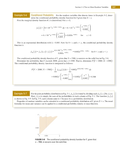
The conditional probability density function of Y, given that X = 1500, is nonzero on the solid line in Fig. 5-8.
(
Determine the probability that Y exceeds 2000, given that x = 1500. That is, determine P Y . 2000 u X 51500) ?
The conditional probability density function is integrated as follows:
(
(
.
P Y . 2000 u X 51500) 5 ∞ ∫ f Y 1500u ( ) ∞ ∫ 0 002 e 0 002 1500) 2 0 0 . 002y dy
y dy 5
.
2000 2000
⎛ e 2 . 0 002y ∞ ⎞ ⎛ e 2 24 ⎞
0 002e ⎜
.
5 . 3 ⎟ 5 . 3 ⎜ ⎟ 5 0 368
0 002e
⎜2 . 2000⎠ ⎟ ⎝ 0 002⎠
0 002
.
⎝
Example 5-7 For the joint probability distribution in Fig. 5-1, f Y x| ( y) is found by dividing each f XY ( x y) by f x).
(
,
x
Here, f x) is simply the sum of the probabilities in each column of Fig. 5-1. The function f Y x| ( y)
(
x
is shown in Fig. 5-9. In Fig. 5-9, each column sums to 1 because it is a probability distribution.
Properties of random variables can be extended to a conditional probability distribution of Y given X = x. The usual
formulas for mean and variance can be applied to a conditional probability density or mass function.
y
1500
0
0 1500 x
FIGURE 5-8 The conditional probability density function for Y , given that
x =1500, is nonzero over the solid line.