Page 180 - Applied statistics and probability for engineers

158 Chapter 5/Joint Probability Distributions

f XY (x, y)

f XY (x, y)
y

R
y
x 7.80 x
3.05
7.70
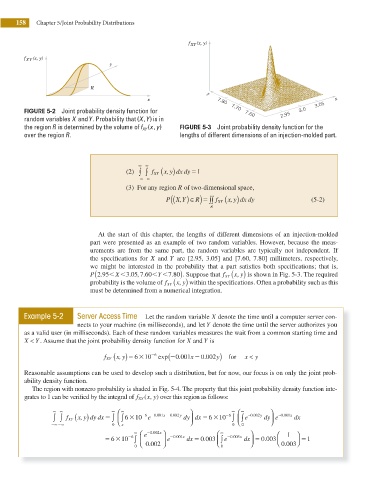
FIGURE 5-2 Joint probability density function for 7.60 2.95 3.0
random variables X and Y . Probability that (X ,Y ) is in
,
the region R is determined by the volume of f XY ( x y) FIGURE 5-3 Joint probability density function for the
over the region R. lengths of different dimensions of an injection-molded part.

∞ ∞
)
(2) ∫ ∫ f XY ( x, y dx dy51
2∞ 2∞
(3) For any region R of two-dimensional space,
( (
)

P X,Y) ∈ R) ∫∫ f XY ( x, y dx dy (5-2)
5
R
At the start of this chapter, the lengths of different dimensions of an injection-molded
part were presented as an example of two random variables. However, because the meas-
urements are from the same part, the random variables are typically not independent. If
the specii cations for X and Y are [2.95, 3.05] and [7.60, 7.80] millimeters, respectively,
we might be interested in the probability that a part satisi es both specii cations; that is,
. (

Y
.
,
.
,
.
,
P 2 95, X 3 05 7 60, , 7 80). Suppose that f XY ( x y) is shown in Fig. 5-3. The required
probability is the volume of f XY ( x y) within the speciications. Often a probability such as this

,

must be determined from a numerical integration.
Example 5-2 Server Access Time Let the random variable X denote the time until a computer server con-
nects to your machine (in milliseconds), and let Y denote the time until the server authorizes you
as a valid user (in milliseconds). Each of these random variables measures the wait from a common starting time and
Y
X < . Assume that the joint probability density function for X and Y is
f XY ( x, y)5 310 26 exp (20 001. x 20 002y ) for x < y
.
6
Reasonable assumptions can be used to develop such a distribution, but for now, our focus is on only the joint prob-
ability density function.
The region with nonzero probability is shaded in Fig. 5-4. The property that this joint probability density function inte-
grates to 1 can be veriied by the integral of f XY ( x y) over this region as follows:
,

∞ ∞ ∞ ⎛ ∞ ⎞ ∞ ⎛ ∞ ⎞
)
∫ ∫ f XY ( x, y dy dx 5 ∫ ⎜ ∫ 6 310 26 e 20 001. x 2 0 002. y dy dx 5 3 10 2 6 ∫ ∫ ⎜ e − . 0 002 y dy e − . x dx
0 001
x
⎟
⎟
6
2∞ 2∞ 0 x ⎝ ⎠ 0 0 ⎝ ⎠
∞ ⎛ e 2 0 0 . 002x ⎞ ⎛ ∞ ⎞ ⎛ 1 ⎞
.
.
5 63 10 2 6 ∫ ⎜ ⎟ e 2 0 001x dx 5 0 003 ⎜ ∫ e 2 0 003x dx 5 0.0003 ⎜ ⎟ 5 1
.
⎟
0 003⎠
0 ⎝ 0 002 ⎠ 0 ⎝ ⎠ ⎝ .
.