Page 183 - Applied statistics and probability for engineers

Section 5-1/Two or More Random Variables 161

y
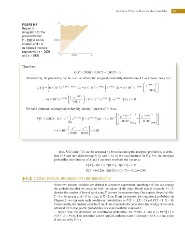
FIGURE 5-7
Region of
integration for the
probability that
Y > 2000 is darkly 2000
shaded, and it is
partitioned into two
regions with x ,2000 0
and x .2000. 0 2000 x

Therefore,
(
P Y . 2000) 50 0475 10 0025 50.
.
.
Alternatively, the probability can be calculated from the marginal probability distribution of Y as follows. For y > 0,
0 001x ⎞
f Y ( y) ∫ y 310 26 e 20 001 x 2 0 002. y dx 5 36 10 26 e 20 002 y ∫ y e 20 001 x dx 5 3 10 e 0 002y ⎛ ⎜ e 2 . y ⎟
2
6 2 .
.
.
.
6
5 6
0 001 ⎟
⎝
0 0 0 ⎜2 . 0⎠
⎛
.
1
.
6 2 .
.
2
5 63 10 e 0 002y 12e . 2 0 001y ⎞ ⎟ 5 63 10 2 3 e 2 0 002y ( 12e 2 0 001y ) for y . 0
⎜
0 001 ⎠
⎝
We have obtained the marginal probability density function of Y. Now,
.
(
P Y . 2000) 5 310 23 ∞ ∫ e 20 002 y 1 ( 2 e 20 001 y ) dy 5 36 10 23 ⎢ ⎛ ⎡ ⎜ e 20 0 . 002y ∞ ⎞ ⎟ 2⎜ ⎛ e 2 0 003y ∞ ⎞ ⎤ ⎥
⎟
.
.
6
.
0 003
⎣ ⎦
2000 ⎜ ⎢ ⎝ 2 0 002 2000⎠ ⎟ ⎜ ⎝ 2 . 2000⎠ ⎟ ⎥ ⎥
⎡ e 24 e 26 ⎤
23
5 310 ⎢ − ⎥ 5 0 05
6
.
.
⎣ 0 002 0 003 ⎦
.
Also, E X) and V X) can be obtained by irst calculating the marginal probability distribu-

(
(
(
(
tion of X and then determining E X) and V X) by the usual method. In Fig. 5-6, the marginal
probability distributions of X and Y are used to obtain the means as
13
.
12
E X ( ) ( ) (0 25 ) (0 55. )52 35.
51 0 2
.
E Y)=1(0.28)+2(0.25)+3(0.177)+4(0.3)=2.49
(
5-1.3 CONDITIONAL PROBABILITY DISTRIBUTIONS
When two random variables are deined in a random experiment, knowledge of one can change

the probabilities that we associate with the values of the other. Recall that in Example 5-1, X
denotes the number of bars of service and Y denotes the response time. One expects the probability
Y51 to be greater at X53 bars than at X51 bar. From the notation for conditional probability in
1)
(
(
Chapter 2, we can write such conditional probabilities as P Y 51u X 53) and P Y 51u X 5 ?
Consequently, the random variables X and Y are expected to be dependent. Knowledge of the value
obtained for X changes the probabilities associated with the values of Y.
Recall that the dei nition of conditional probability for events A and B is P B Au ( ) =
(
P A> B) / P A). This dei nition can be applied with the event A dei ned to be X = x and event
(
B deined to be Y = y.